Results in a plot to check whether the propensity score has adequate overlap between treatment groups
Arguments
- x
The design matrix (not including intercept term)
- trt
treatment vector with each element equal to a 0 or a 1, with 1 indicating treatment status is active.
- propensity.func
function that inputs the design matrix x and the treatment vector trt and outputs the propensity score, ie Pr(trt = 1 | X = x). Function should take two arguments 1) x and 2) trt. See example below. For a randomized controlled trial this can simply be a function that returns a constant equal to the proportion of patients assigned to the treatment group, i.e.:
propensity.func = function(x, trt) 0.5.- type
Type of plot to create. Options are either a histogram (
type = "histogram") for each treatment group, a density (type = "density") for each treatment group, or to plot both a density and histogram (type = "code")- bins
integer number of bins for histograms when
type = "histogram"- alpha
value between 0 and 1 indicating transparency level (1 for solid, 0 for fully transparent)
Examples
library(personalized)
set.seed(123)
n.obs <- 250
n.vars <- 15
x <- matrix(rnorm(n.obs * n.vars, sd = 3), n.obs, n.vars)
# simulate non-randomized treatment
xbetat <- 0.25 + 0.5 * x[,11] - 0.5 * x[,12]
trt.prob <- exp(xbetat) / (1 + exp(xbetat))
trt01 <- rbinom(n.obs, 1, prob = trt.prob)
# create function for fitting propensity score model
prop.func <- function(x, trt)
{
# fit propensity score model
propens.model <- cv.glmnet(y = trt,
x = x, family = "binomial")
pi.x <- predict(propens.model, s = "lambda.min",
newx = x, type = "response")[,1]
pi.x
}
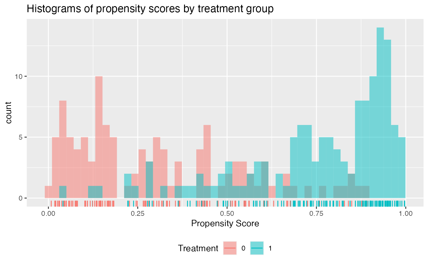
check.overlap(x = x,
trt = trt01,
propensity.func = prop.func)
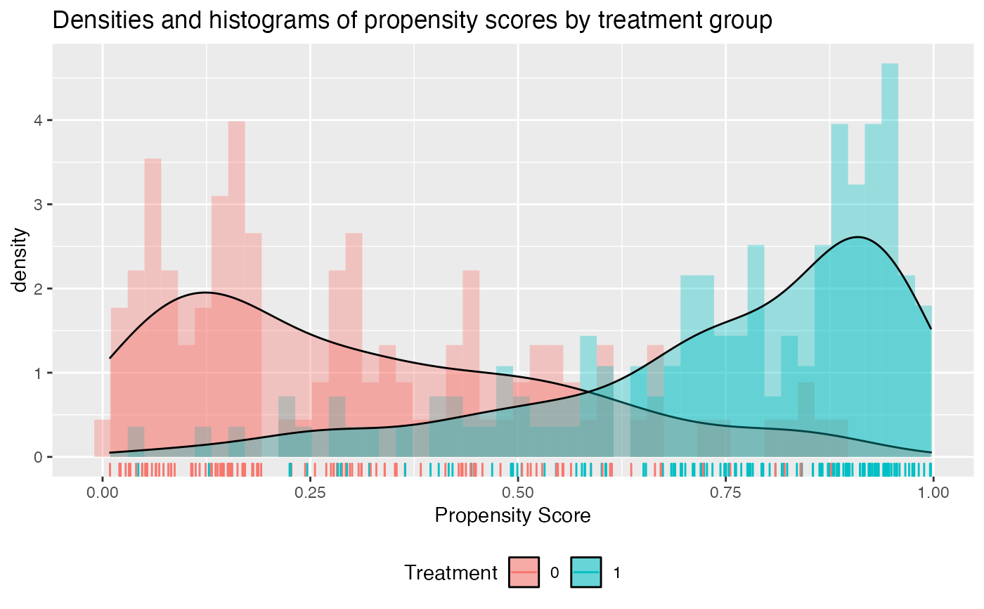
 # now add density plot with histogram
check.overlap(x = x,
trt = trt01,
type = "both",
propensity.func = prop.func)
# now add density plot with histogram
check.overlap(x = x,
trt = trt01,
type = "both",
propensity.func = prop.func)
 # simulated non-randomized treatment with multiple levels
xbetat_1 <- 0.15 + 0.5 * x[,9] - 0.25 * x[,12]
xbetat_2 <- 0.15 - 0.5 * x[,11] + 0.25 * x[,15]
trt.1.prob <- exp(xbetat_1) / (1 + exp(xbetat_1) + exp(xbetat_2))
trt.2.prob <- exp(xbetat_2) / (1 + exp(xbetat_1) + exp(xbetat_2))
trt.3.prob <- 1 - (trt.1.prob + trt.2.prob)
prob.mat <- cbind(trt.1.prob, trt.2.prob, trt.3.prob)
trt <- apply(prob.mat, 1, function(rr) rmultinom(1, 1, prob = rr))
trt <- apply(trt, 2, function(rr) which(rr == 1))
# use multinomial logistic regression model with lasso penalty for propensity
propensity.multinom.lasso <- function(x, trt)
{
if (!is.factor(trt)) trt <- as.factor(trt)
gfit <- cv.glmnet(y = trt, x = x, family = "multinomial")
# predict returns a matrix of probabilities:
# one column for each treatment level
propens <- drop(predict(gfit, newx = x, type = "response", s = "lambda.min",
nfolds = 5, alpha = 0))
# return the probability corresponding to the
# treatment that was observed
probs <- propens[,match(levels(trt), colnames(propens))]
probs
}
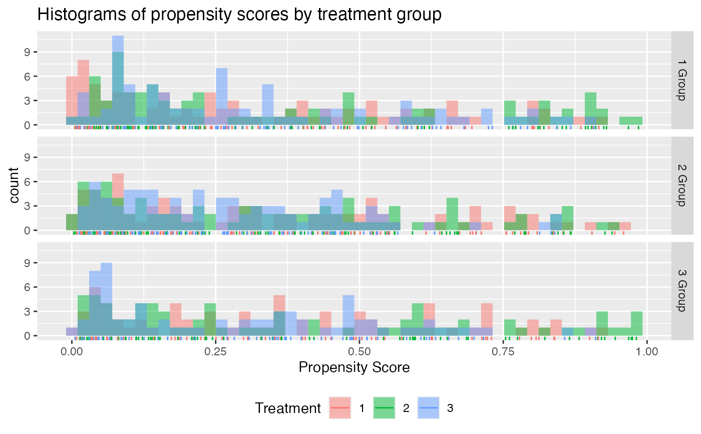
check.overlap(x = x,
trt = trt,
type = "histogram",
propensity.func = propensity.multinom.lasso)
# simulated non-randomized treatment with multiple levels
xbetat_1 <- 0.15 + 0.5 * x[,9] - 0.25 * x[,12]
xbetat_2 <- 0.15 - 0.5 * x[,11] + 0.25 * x[,15]
trt.1.prob <- exp(xbetat_1) / (1 + exp(xbetat_1) + exp(xbetat_2))
trt.2.prob <- exp(xbetat_2) / (1 + exp(xbetat_1) + exp(xbetat_2))
trt.3.prob <- 1 - (trt.1.prob + trt.2.prob)
prob.mat <- cbind(trt.1.prob, trt.2.prob, trt.3.prob)
trt <- apply(prob.mat, 1, function(rr) rmultinom(1, 1, prob = rr))
trt <- apply(trt, 2, function(rr) which(rr == 1))
# use multinomial logistic regression model with lasso penalty for propensity
propensity.multinom.lasso <- function(x, trt)
{
if (!is.factor(trt)) trt <- as.factor(trt)
gfit <- cv.glmnet(y = trt, x = x, family = "multinomial")
# predict returns a matrix of probabilities:
# one column for each treatment level
propens <- drop(predict(gfit, newx = x, type = "response", s = "lambda.min",
nfolds = 5, alpha = 0))
# return the probability corresponding to the
# treatment that was observed
probs <- propens[,match(levels(trt), colnames(propens))]
probs
}
check.overlap(x = x,
trt = trt,
type = "histogram",
propensity.func = propensity.multinom.lasso)