Stagewise Variable Selection for Joint Semi-Competing Risk Models

Overview

The swjm package implements stagewise variable selection for joint models of semi-competing risks. In many medical settings — such as hospital readmission following discharge — patients can experience a non-terminal recurrent event (readmission) and a terminal event (death). Death precludes future readmissions, but readmission does not preclude death, a structure known as semi-competing risks.

Two joint model frameworks are supported:

Model	Type	Recurrence process	Terminal process
JFM	Joint Frailty Model (Cox)	Proportional hazards	Proportional hazards
JSCM	Joint Scale-Change Model (AFT)	Rank-based estimating equations	Rank-based estimating equations

Three penalty types are available: cooperative lasso ("coop"), lasso ("lasso"), and group lasso ("group"). The cooperative lasso is the recommended default; it encourages predictors that affect both outcomes to enter together with the same sign.

1. Statistical Background

1.1 Semi-Competing Risks

Let $N_i^R(t)$ count the readmission events for subject $i$ by time $t$ , and let $T_i^D$ denote the time to death. Death censors future readmissions; readmission does not censor death.

Each subject $i$ ( $i = 1, \ldots, n$ ) has:

A $p$ -dimensional covariate vector $Z_i$ (possibly time-varying).
An observed follow-up interval $[0, C_i]$ where $C_i$ is the censoring time.

The parameter vector of interest is $\theta = (\alpha^\top, \beta^\top)^\top \in \mathbb{R}^{2p},$ where $\alpha \in \mathbb{R}^p$ governs the recurrence (readmission) process and $\beta \in \mathbb{R}^p$ governs the terminal (death) process.

1.2 Joint Frailty Model (JFM)

The JFM (Kalbfleisch et al., 2013) introduces a subject-specific frailty $\omega_i \sim \text{Gamma}(\kappa, \kappa)$ that links the two processes:

$\lambda^R(t \mid Z_i, \omega_i) = \lambda_0^R(t)\, e^{\alpha^\top Z_i(t)}\, \omega_i, \qquad \lambda^D(t \mid Z_i, \omega_i) = \lambda_0^D(t)\, e^{\beta^\top Z_i}\, \omega_i^\eta,$

where $\lambda_0^R$ and $\lambda_0^D$ are unspecified baseline hazard functions. Marginalising over $\omega_i$ yields estimating equations that are functions only of $(\alpha, \beta)$ and the two baseline hazards.

In the package, alpha is always the readmission coefficient vector and beta is always the death coefficient vector.

1.3 Joint Scale-Change Model (JSCM)

The JSCM (Xu et al.) replaces proportional hazards with an AFT-type scale-change specification:

$\lambda^R(t \mid Z_i) = e^{\alpha^\top Z_i}\, \lambda_0^R(t\,e^{\alpha^\top Z_i}), \qquad \lambda^D(t \mid Z_i) = e^{\beta^\top Z_i}\, \lambda_0^D(t\,e^{\beta^\top Z_i}).$

Estimation is based on rank-based estimating equations implemented in C++ via RcppArmadillo.

1.4 Stagewise Variable Selection

The goal is to find a sparse $\theta$ that minimizes a penalized estimating equation criterion. Three penalty structures are supported:

Scaled lasso (independent selection): $\text{pen}(\theta;\lambda) = \lambda \sum_{j=1}^p \left(\frac{|\alpha_j|}{s_\alpha} + \frac{|\beta_j|}{s_\beta}\right),$

Group lasso (simultaneous entry of $(\alpha_j, \beta_j)$ pairs): $\text{pen}(\theta;\lambda) = \lambda \sum_{j=1}^p \left\|\left(\frac{\alpha_j}{s_\alpha}, \frac{\beta_j}{s_\beta}\right)\right\|_2,$

Cooperative lasso (encourages shared sign and support): $\text{pen}(\theta;\lambda) = \lambda \sum_{j=1}^p \begin{cases} \left\|\left(\frac{\alpha_j}{s_\alpha}, \frac{\beta_j}{s_\beta}\right)\right\|_2 & \text{if } \text{sgn}(\alpha_j) = \text{sgn}(\beta_j), \\[6pt] \left\|\left(\frac{\alpha_j}{s_\alpha}, \frac{\beta_j}{s_\beta}\right)\right\|_\infty & \text{if } \text{sgn}(\alpha_j) \ne \text{sgn}(\beta_j). \end{cases}$

The cooperative lasso uses the L2 norm when both coefficients agree in sign (rewarding variables that affect both outcomes in the same direction) and the L-infinity norm when they disagree (applying a harsher penalty).

The stagewise algorithm approximates the penalized solution by taking small gradient steps in the direction determined by the dual norm of the current estimating equation score. At each iteration:

Compute the EE score $U(\theta)$ (gradient of the unpenalized estimating equation objective).
Find the active coordinate(s) with the largest penalized dual norm.
Update $\theta$ by a small step $\epsilon$ in that direction.

The regularization path is indexed by $\lambda$ , recorded as the dual norm at each step. Cross-validation over a grid of $\lambda$ values selects the optimal tuning parameter.

1.5 Cross-Validation

cv_stagewise() performs stratified K-fold cross-validation. For each fold, it evaluates the cross-fitted EE score norm — the score from the held-out fold evaluated at the coefficient fit from the remaining folds. The optimal $\lambda$ minimizes the total cross-fitted norm across both sub-models.

2. Installation

# From the package source directory:
devtools::install("swjm")

# Or from a built tarball:
install.packages("swjm_0.1.0.tar.gz", repos = NULL, type = "source")

3. Data Format

All functions expect a data frame in counting-process (interval) format with the following required columns:

Column	Description
`id`	Subject identifier
`t.start`	Interval start time
`t.stop`	Interval end time
`event`	1 = readmission (recurrent event), 0 = death/censoring row
`status`	1 = death, 0 = alive/censored
`x1, …, xp`	Covariate columns

Each subject contributes multiple rows:

One row per readmission interval (with event = 1), followed by
One terminal row (with event = 0) recording either death (status = 1) or censoring (status = 0).

The covariate values may differ across rows for the same subject (JFM supports time-varying covariates; JSCM uses the baseline values from the event = 0 rows).

4. Simulating Data

generate_data() is a unified data-generation interface for both models.

library(swjm)

4.1 Joint Frailty Model data

set.seed(123)
dat_jfm  <- generate_data(n = 500, p = 10, scenario = 1, model = "jfm")
Data_jfm <- dat_jfm$data

# Preview
head(Data_jfm[, 1:8])
#>   id   t.start    t.stop event status         x1          x2         x3
#> 1  1 0.0000000 0.1847740     1      0 -0.3756029 -0.56187636 -0.3439172
#> 2  1 0.1847740 2.5816764     0      0 -0.4898705  0.04715443  1.3001987
#> 3  2 0.0000000 0.2965848     1      0  0.6843094 -1.39527435  0.8496430
#> 4  2 0.2965848 1.6792116     1      0 -0.2656516  0.11814451  0.1340386
#> 5  2 1.6792116 1.7574405     1      0  2.0024827  0.06670087  1.8668518
#> 6  2 1.7574405 1.8132809     1      0  0.3311792 -2.01421050  0.2119804

JFM: 500 subjects, 1513 rows, 1013 readmissions, 104 deaths

The returned list also contains the true generating coefficients:

True alpha (readmission):

round(dat_jfm$alpha_true, 2)
#>  [1]  1.1 -1.1  0.1 -0.1  0.0  0.0  0.0  0.0  1.0 -1.0

True beta (death):

round(dat_jfm$beta_true, 2)
#>  [1]  0.1 -0.1  1.1 -1.1  0.0  0.0  0.0  0.0  1.0 -1.0

Scenario descriptions (for both JFM and JSCM):

Scenario	Signal structure
1	Variables affecting readmission only, death only, and both processes
2	Larger block of shared-sign signals
3	Mixed-sign signals (some variables have opposite effects on the two outcomes)

4.2 Joint Scale-Change Model data

set.seed(456)
dat_jscm  <- generate_data(n = 500, p = 10, scenario = 1, model = "jscm")
#> Call: 
#> reReg::simGSC(n = n, summary = TRUE, para = para, xmat = X, censoring = C, 
#>     frailty = gamma, tau = 60)
#> 
#> Summary:
#> Sample size:                                    500 
#> Number of recurrent event observed:             937 
#> Average number of recurrent event per subject:  1.874 
#> Proportion of subjects with a terminal event:   0.212
Data_jscm <- dat_jscm$data

JSCM: 500 subjects, 1437 rows, 937 readmissions, 106 deaths

For the JSCM, covariates are drawn from $\text{Uniform}(-1, 1)$ , and a gamma frailty ( $\text{shape} = 4$ , $\text{scale} = 0.25$ ) is used in simulation. Censoring times are $\text{Uniform}(0, 4)$ .

5. Joint Frailty Model (JFM) Workflow

5.1 Fit the Stagewise Regularization Path

stagewise_fit() traces the full coefficient path as $\lambda$ decreases from a large value (all coefficients zero) to a small value (many active variables):

fit_jfm <- stagewise_fit(
  Data_jfm,
  model   = "jfm",
  penalty = "coop"    # cooperative lasso
)
fit_jfm
#> Stagewise path (jfm/coop)
#> 
#>   Covariates (p):            10
#>   Iterations:                5000
#>   Lambda range:              [0.03849, 1.442]
#>   Active at final step:      10 readmission, 10 death
#>     Readmission (alpha): 1, 2, 3, 4, 5, 6, 7, 8, 9, 10
#>     Death (beta):        1, 2, 3, 4, 5, 6, 7, 8, 9, 10

The returned swjm_path object contains:

Component	Description
`alpha`	$p \times (k+1)$ matrix of readmission coefficients along the path
`beta`	$p \times (k+1)$ matrix of death coefficients along the path
`theta`	$2p \times (k+1)$ combined matrix (`rbind(alpha, beta)`)
`lambda`	Dual norm at each step (regularization path index)
`model`	`"jfm"` or `"jscm"`
`penalty`	`"coop"`, `"lasso"`, or `"group"`
`p`	Number of covariates

5.2 Explore the Regularization Path

p <- 10
k <- ncol(fit_jfm$alpha)
active_final <- which(fit_jfm$alpha[, k] != 0 |
                      fit_jfm$beta[, k]  != 0)

Path length: 5001 steps
Lambda range: [0.03849, 1.442]
Active variables at final step: 1 2 3 4 5 6 7 8 9 10

Readmission (alpha) coefficients at the final step:

round(fit_jfm$alpha[, k], 4)
#>  [1]  1.1049 -1.0964  0.1198 -0.0414  0.0016  0.0003  0.0121  0.0037  0.9539
#> [10] -0.9847

summary() shows a compact table of path-end coefficients annotated with variable type (shared, readmission-only, or death-only):

summary(fit_jfm)
#> Stagewise path (jfm/coop)
#> 
#>   p = 10  |  5000 iterations  |  lambda: [0.03849, 1.442]
#>   Decreasing path: 604 steps
#> 
#>   Path-end coefficients (nonzero variables):
#> 
#>   Variable    alpha       beta        Type
#>   ----------  ----------  ----------  ----------------
#>   x10         -0.9847     -0.9070     shared (+)
#>   x3          +0.1198     +1.1685     shared (+)
#>   x9          +0.9539     +0.9246     shared (+)
#>   x1          +1.1049     +0.2680     shared (+)
#>   x2          -1.0964     -0.0318     shared (+)
#>   x4          -0.0414     -1.1720     shared (+)
#>   x8          +0.0037     +0.0829     shared (+)
#>   x5          +0.0016     +0.0128     shared (+)
#>   x7          +0.0121     +0.0120     shared (+)
#>   x6          +0.0003     -0.0091     shared (–)

5.3 Plot the Coefficient Path

plot() produces a glmnet-style coefficient trajectory plot. Two panels are drawn by default — one for readmission ( $\alpha$ ) and one for death ( $\beta$ ) — with the number of active variables on the top axis.

plot(fit_jfm)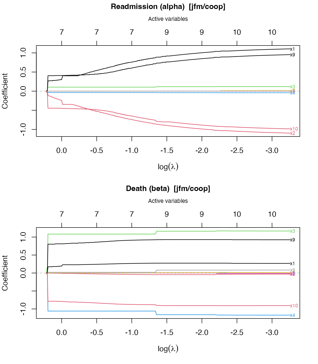

To plot only one sub-model:

plot(fit_jfm, which = "readmission")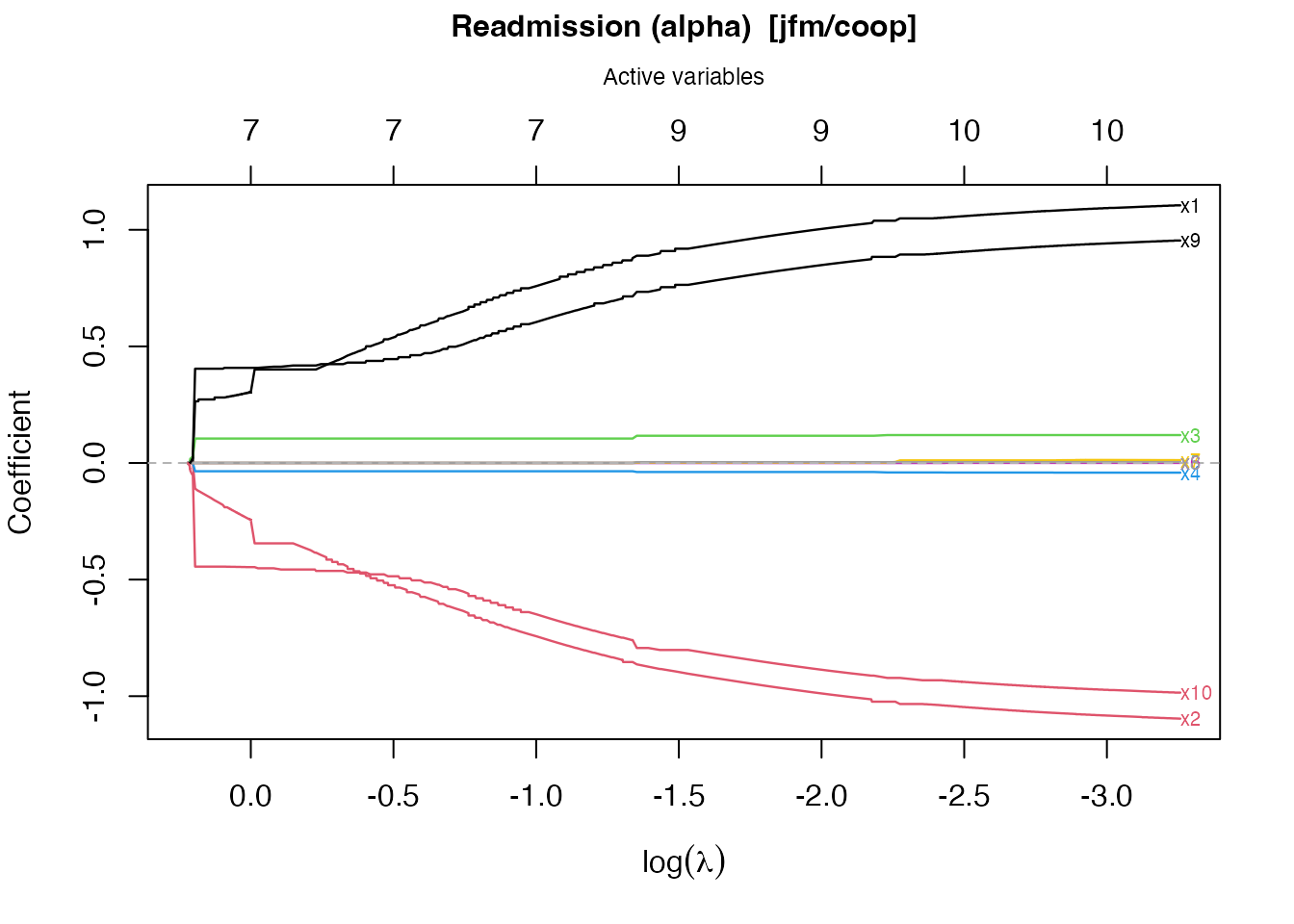

5.4 Cross-Validation

cv_stagewise() selects the optimal $\lambda$ by K-fold cross-validation using cross-fitted EE score norms.

It is good practice to restrict the $\lambda$ grid to the strictly decreasing portion of the path (using extract_decreasing_indices()):

lambda_path <- fit_jfm$lambda
dec_idx     <- swjm:::extract_decreasing_indices(lambda_path)
lambda_seq  <- lambda_path[dec_idx]

Full path: 5001 steps; decreasing path: 604 steps

set.seed(1)
cv_jfm <- cv_stagewise(
  Data_jfm,
  model      = "jfm",
  penalty    = "coop",
  lambda_seq = lambda_seq,
  K          = 3L
)
cv_jfm
#> Cross-validation (jfm/coop)
#> 
#>   Covariates (p):              10
#>   Lambda grid size:            604
#>   Best position (combined):    604  (lambda = 0.03849)
#>   Selected variables:          10 readmission, 10 death
#>     Readmission (alpha): 1, 2, 3, 4, 5, 6, 7, 8, 9, 10
#>     Death (beta):        1, 2, 3, 4, 5, 6, 7, 8, 9, 10

The returned swjm_cv object contains:

Component	Description
`alpha`	Readmission coefficients at the optimal $\lambda$
`beta`	Death coefficients at the optimal $\lambda$
`position_CF`	Index of optimal $\lambda$ in `lambda_seq`
`lambda_seq`	The $\lambda$ grid used for cross-validation
`Scorenorm_crossfit`	Combined cross-fitted EE norm over the grid
`Scorenorm_crossfit_re`	Readmission component
`Scorenorm_crossfit_ce`	Death component
`n_active_alpha`	Number of active readmission variables per $\lambda$
`n_active_beta`	Number of active death variables per $\lambda$
`n_active`	Total active variables
`baseline`	Cumulative baseline hazards (Breslow for JFM; Nelson-Aalen on accelerated scale for JSCM)

The optimal $\lambda$ is cv_jfm$lambda_seq[cv_jfm$position_CF].

5.5 Plot the CV Results

plot(cv_jfm)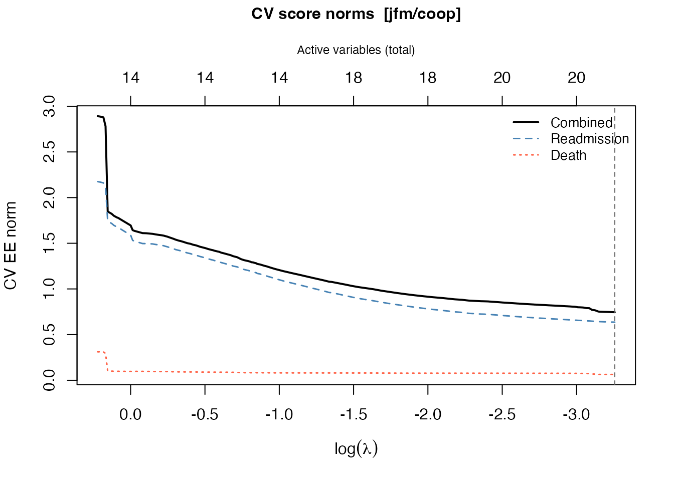

The plot shows three curves: the combined norm (black, solid), the readmission component (blue, dashed), and the death component (red, dotted). The vertical dashed line marks the optimal $\lambda$ .

5.6 Extract Coefficients and Summarize

Selected readmission (alpha) variables: 1 2 3 4 5 6 7 8 9 10

Selected death (beta) variables: 1 2 3 4 5 6 7 8 9 10

Nonzero alpha:

round(cv_jfm$alpha[cv_jfm$alpha != 0], 4)
#>  [1]  1.1049 -1.0964  0.1198 -0.0414  0.0016  0.0003  0.0122  0.0037  0.9539
#> [10] -0.9847

Nonzero beta:

round(cv_jfm$beta[cv_jfm$beta != 0], 4)
#>  [1]  0.2680 -0.0318  1.1685 -1.1720  0.0128 -0.0091  0.0120  0.0829  0.9246
#> [10] -0.9070

summary() shows a formatted table with the CV-optimal coefficients:

summary(cv_jfm)
#> CV-selected model (jfm/coop)
#> 
#>   p = 10  |  Lambda grid: 604 steps  |  CV optimal: step 604 (lambda = 0.03849)
#> 
#>   Selected coefficients  (10 readmission, 10 death):
#> 
#>   Variable    alpha       beta        Type
#>   ----------  ----------  ----------  ----------------
#>   x10         -0.9847     -0.9070     shared (+)
#>   x9          +0.9539     +0.9246     shared (+)
#>   x1          +1.1049     +0.2680     shared (+)
#>   x3          +0.1198     +1.1685     shared (+)
#>   x4          -0.0414     -1.1720     shared (+)
#>   x2          -1.0964     -0.0318     shared (+)
#>   x8          +0.0037     +0.0829     shared (+)
#>   x7          +0.0122     +0.0120     shared (+)
#>   x5          +0.0016     +0.0128     shared (+)
#>   x6          +0.0003     -0.0091     shared (–)

coef() returns the combined $2p$ -vector c(alpha, beta) for programmatic use:

theta_best <- coef(cv_jfm)
length(theta_best)  # 2p
#> [1] 20

5.7 Baseline Hazard

baseline_hazard() evaluates the cumulative baseline hazards at specified time points. For JFM, Breslow-type estimators are used:

bh <- baseline_hazard(cv_jfm, times = c(0.5, 1.0, 2.0, 4.0, 6.0))
print(bh)
#>   time cumhaz_readmission cumhaz_death
#> 1  0.5          0.5130553   0.01761970
#> 2  1.0          1.0383574   0.03233941
#> 3  2.0          1.9661915   0.07509280
#> 4  4.0          3.9035132   0.14598819
#> 5  6.0          5.4918966   0.19762732

To retrieve only one of the two processes:

bh_re <- baseline_hazard(cv_jfm, times = seq(0, 5, by = 0.5),
                         which = "readmission")
head(bh_re)
#>   time cumhaz_readmission
#> 1  0.0          0.0000000
#> 2  0.5          0.5130553
#> 3  1.0          1.0383574
#> 4  1.5          1.5229562
#> 5  2.0          1.9661915
#> 6  2.5          2.4650482

5.8 Survival Prediction

predict() computes subject-specific survival curves for both readmission and death. For JFM, Breslow cumulative baseline hazards are used: $S_{\text{re}}(t \mid z) = \exp\!\bigl(-\hat\Lambda_0^r(t)\, e^{\hat\alpha^\top z}\bigr), \qquad S_{\text{de}}(t \mid z) = \exp\!\bigl(-\hat\Lambda_0^d(t)\, e^{\hat\beta^\top z}\bigr).$ For JSCM, Nelson-Aalen baselines on the accelerated time scale are used (see Section 7.5).

set.seed(7)
newz <- matrix(rnorm(30), nrow = 3, ncol = 10)
rownames(newz) <- paste0("Patient_", 1:3)
colnames(newz) <- paste0("x", 1:10)

pred <- predict(cv_jfm, newdata = newz)
pred
#> swjm predictions (jfm)
#> 
#>   Subjects:                3
#>   Time points:             1117
#>   Time range:              [8.134e-05, 6.153]
#> 
#>   Use plot() to visualize survival curves and predictor contributions.

The swjm_pred object contains:

S_re: readmission-free survival matrix (subjects × time points)
S_de: death-free survival matrix
lp_re: linear predictors $\hat\alpha^\top z_i$
lp_de: linear predictors $\hat\beta^\top z_i$
contrib_re, contrib_de: per-predictor contributions $\hat\alpha_j z_{ij}$

# Survival probabilities for all subjects at first few time points
round(pred$S_re[, 1:5], 3)
#>           t=8.134e-05 t=0.0002363 t=0.0002812 t=0.0003871 t=0.0006399
#> Patient_1       0.991       0.991       0.983       0.975       0.966
#> Patient_2       0.999       0.999       0.999       0.998       0.998
#> Patient_3       0.999       0.999       0.999       0.998       0.997

plot() on a swjm_pred object produces a four-panel figure: survival curves for both processes (all subjects in grey, highlighted subject in color) plus bar charts of predictor contributions:

plot(pred, which_subject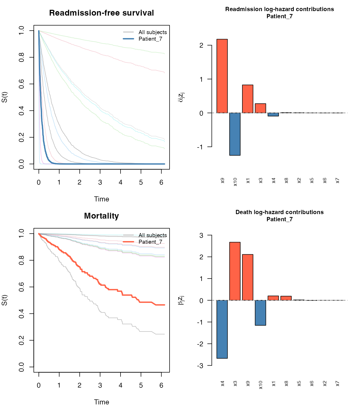 = 1)

To focus on only one process:

plot(pred, which_subject = 2, which_process = "readmission")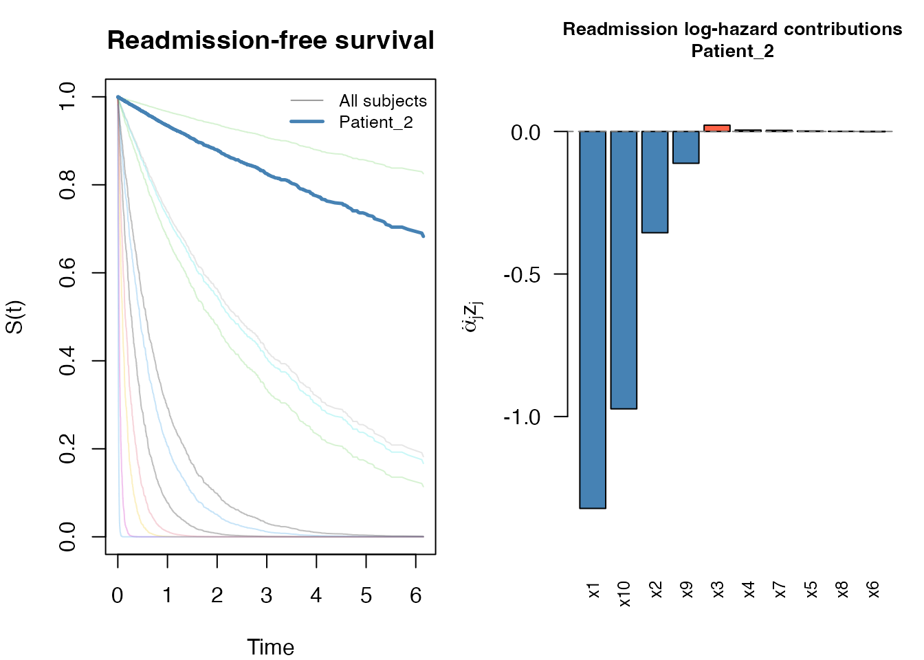

6. Other Penalty Types (JFM)

All three penalties are available for both models. Here we illustrate the lasso and group lasso on the JFM data.

6.1 Lasso

The lasso penalizes each coordinate independently. It allows variables to enter the readmission path without entering the death path (and vice versa):

fit_lasso <- stagewise_fit(Data_jfm, model = "jfm", penalty = "lasso")
set.seed(2)
cv_lasso <- cv_stagewise(Data_jfm, model = "jfm", penalty = "lasso", K = 3L)
summary(cv_lasso)

6.2 Group Lasso

The group lasso treats $(\alpha_j, \beta_j)$ pairs as groups; a variable enters (or leaves) both sub-models simultaneously:

fit_group <- stagewise_fit(Data_jfm, model = "jfm", penalty = "group")
set.seed(3)
cv_group <- cv_stagewise(Data_jfm, model = "jfm", penalty = "group", K = 3L)
summary(cv_group)

6.3 Comparing Penalties

The cooperative lasso typically achieves better variable selection than the standard lasso when the true signal is sparse and shared between outcomes. The group lasso is a good alternative when you expect all relevant predictors to affect both outcomes with comparable magnitude.

7. Joint Scale-Change Model (JSCM) Workflow

The JSCM workflow mirrors the JFM workflow with two differences:

The default step size is smaller (eps = 0.01) and more iterations are needed (max_iter = 5000).
The EE is rank-based (implemented in C++ via RcppArmadillo).
Survival curves are computed via a Nelson-Aalen estimator on the accelerated time scale. For subject $i$ with linear predictor $\hat\alpha^\top z_i$ , the recurrence survival function is $S_{\text{re}}(t \mid z_i) = \exp\!\bigl(-\hat\Lambda_0^r(t\, e^{\hat\alpha^\top z_i})\bigr)$ , where $\hat\Lambda_0^r$ is estimated by pooling all accelerated event times $t_{ij}\,e^{\hat\alpha^\top z_i}$ .

7.1 Fit the Stagewise Path

set.seed(456)
dat_jscm  <- generate_data(n = 500, p = 10, scenario = 1, model = "jscm")
#> Call: 
#> reReg::simGSC(n = n, summary = TRUE, para = para, xmat = X, censoring = C, 
#>     frailty = gamma, tau = 60)
#> 
#> Summary:
#> Sample size:                                    500 
#> Number of recurrent event observed:             937 
#> Average number of recurrent event per subject:  1.874 
#> Proportion of subjects with a terminal event:   0.212
Data_jscm <- dat_jscm$data

fit_jscm <- stagewise_fit(Data_jscm, model = "jscm", penalty = "coop")
fit_jscm
#> Stagewise path (jscm/coop)
#> 
#>   Covariates (p):            10
#>   Iterations:                5000
#>   Lambda range:              [0.0007715, 2.501]
#>   Active at final step:      10 readmission, 10 death
#>     Readmission (alpha): 1, 2, 3, 4, 5, 6, 7, 8, 9, 10
#>     Death (beta):        1, 2, 3, 4, 5, 6, 7, 8, 9, 10

7.2 Cross-Validation

lambda_path_jscm <- fit_jscm$lambda
dec_idx_jscm     <- swjm:::extract_decreasing_indices(lambda_path_jscm)
lambda_seq_jscm  <- lambda_path_jscm[dec_idx_jscm]

set.seed(10)
cv_jscm <- cv_stagewise(
  Data_jscm,
  model      = "jscm",
  penalty    = "coop",
  lambda_seq = lambda_seq_jscm,
  K          = 3L
)
cv_jscm
#> Cross-validation (jscm/coop)
#> 
#>   Covariates (p):              10
#>   Lambda grid size:            457
#>   Best position (combined):    339  (lambda = 0.06191)
#>   Selected variables:          10 readmission, 10 death
#>     Readmission (alpha): 1, 2, 3, 4, 5, 6, 7, 8, 9, 10
#>     Death (beta):        1, 2, 3, 4, 5, 6, 7, 8, 9, 10

7.3 Results

Selected alpha (readmission): 1 2 3 4 5 6 7 8 9 10

Selected beta (death): 1 2 3 4 5 6 7 8 9 10

True nonzero alpha: 1 2 3 4 9 10

True nonzero beta: 1 2 3 4 9 10

plot(cv_jscm)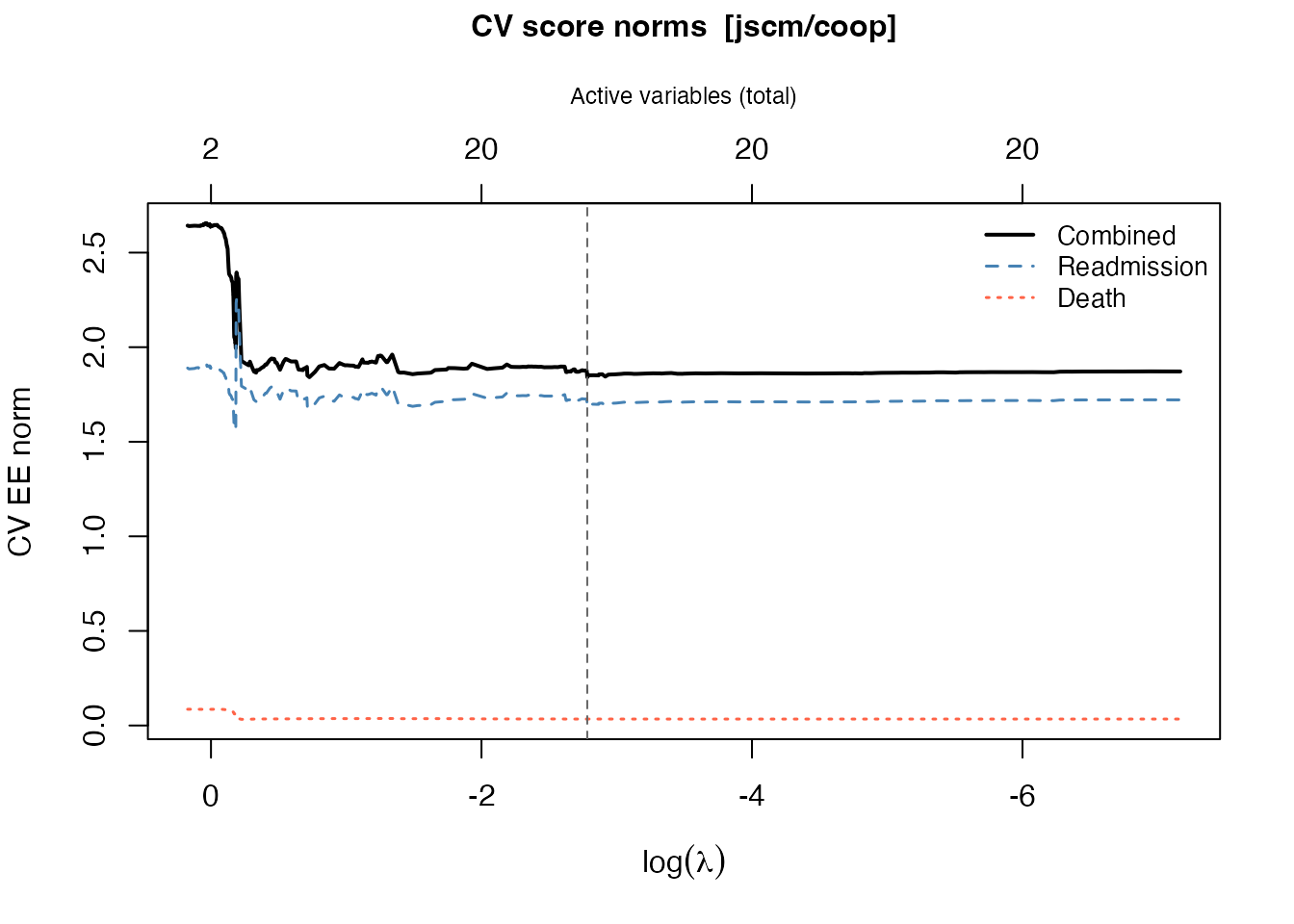

summary(cv_jscm)
#> CV-selected model (jscm/coop)
#> 
#>   p = 10  |  Lambda grid: 457 steps  |  CV optimal: step 339 (lambda = 0.06191)
#> 
#>   Selected coefficients  (10 readmission, 10 death):
#> 
#>   Variable    alpha       beta        Type
#>   ----------  ----------  ----------  ----------------
#>   x10         -1.0864     -1.9254     shared (+)
#>   x3          +0.4167     +1.9260     shared (+)
#>   x9          +1.1099     +0.8149     shared (+)
#>   x1          +1.3184     +0.1840     shared (+)
#>   x4          -0.0208     -1.1301     shared (+)
#>   x2          -0.8731     -0.0591     shared (+)
#>   x7          -0.2715     -0.4874     shared (+)
#>   x5          -0.1978     -0.3748     shared (+)
#>   x6          +0.1109     +0.1221     shared (+)
#>   x8          +0.0212     -0.0100     shared (–)

7.4 Baseline Hazard (JSCM)

baseline_hazard() works for the JSCM as well. The baseline is estimated via Nelson-Aalen on the accelerated time scale: each subject’s event times are multiplied by their acceleration factor $e^{\hat\alpha^\top z_i}$ before pooling, so the resulting $\hat\Lambda_0^r$ is on the common (baseline) time scale.

bh_jscm <- baseline_hazard(cv_jscm, times = c(0.5, 1.0, 2.0, 3.0, 4.0))
print(bh_jscm)
#>   time cumhaz_readmission cumhaz_death
#> 1  0.5          0.7784166   0.08409819
#> 2  1.0          1.2758373   0.12605781
#> 3  2.0          2.0931603   0.20165682
#> 4  3.0          2.6516282   0.27129419
#> 5  4.0          3.1209841   0.31870653

7.5 Survival Prediction and AFT Interpretation

predict() returns subject-specific survival curves for both processes via: $S_{\text{re}}(t \mid z_i) = \exp\!\bigl(-\hat\Lambda_0^r(t\,e^{\hat\alpha^\top z_i})\bigr), \qquad S_{\text{de}}(t \mid z_i) = \exp\!\bigl(-\hat\Lambda_0^d(t\,e^{\hat\beta^\top z_i})\bigr).$

The linear predictor $\hat\alpha^\top z_i$ is a log time-acceleration factor: $e^{\hat\alpha^\top z_i} > 1$ means events are expected sooner than baseline; $< 1$ means later. Each term $e^{\hat\alpha_j z_{ij}}$ is the multiplicative contribution of predictor $j$ :

Value of $e^{\hat\alpha_j z_{ij}}$	Interpretation
$> 1$	predictor $j$ accelerates events — shorter time to readmission
$= 1$	no effect on this subject’s timing
$< 1$	predictor $j$ decelerates events — longer time to readmission

set.seed(7)
newz_jscm <- matrix(runif(30, -1, 1), nrow = 3, ncol = 10)
rownames(newz_jscm) <- paste0("Patient_", 1:3)

pred_jscm <- predict(cv_jscm, newdata = newz_jscm)
pred_jscm
#> swjm predictions (jscm)
#> 
#>   Subjects:                3
#>   Time points:             1043
#>   Time range:              [0.0005412, 88.64]
#> 
#>   Time-acceleration factors (exp(alpha^T z) for recurrence):
#> Patient_1 Patient_2 Patient_3 
#>   12.7055    0.3299    0.2571 
#> 
#>   Time-acceleration factors (exp(beta^T z) for death):
#> Patient_1 Patient_2 Patient_3 
#>    0.7906    1.6779    0.7063 
#> 
#>   Use plot() to visualize survival curves and predictor contributions.

Recurrence time-acceleration factors (total per subject):

round(pred_jscm$time_accel_re, 3)
#> Patient_1 Patient_2 Patient_3 
#>    12.706     0.330     0.257

plot() produces the same four-panel layout as for the JFM: survival curves for both processes (all subjects in grey, highlighted subject in color) plus bar charts of log time-acceleration contributions. The survival panel titles show each subject’s total acceleration factor.

plot(pred_jscm, which_subject = 1)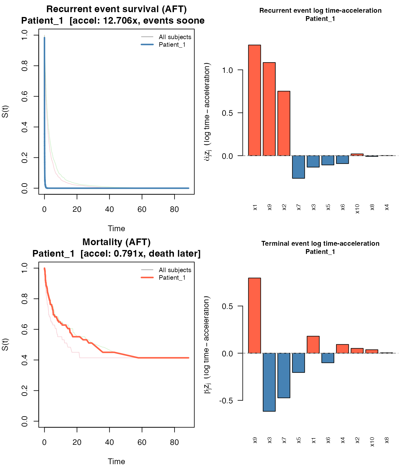

8. Interpreting Output

8.1 Alpha and Beta Conventions

In both JFM and JSCM, alpha governs the recurrence (readmission) process and beta governs the terminal (death) process. The interpretation of the coefficients differs by model:

JFM (proportional hazards):

alpha[j] > 0: covariate $j$ increases the recurrence hazard — more frequent readmissions for higher values of $x_j$ .
beta[j] > 0: covariate $j$ increases the death hazard.
The subject-specific contribution $\hat\alpha_j z_{ij}$ is an additive log-hazard-ratio contribution. Positive = higher risk; negative = lower risk.

JSCM (scale-change / AFT-type):

alpha[j] > 0: covariate $j$ accelerates the recurrence process — events happen sooner for higher values of $x_j$ .
beta[j] > 0: covariate $j$ accelerates the terminal process.
The subject-specific contribution $\hat\alpha_j z_{ij}$ is an additive log time-acceleration contribution. Exponentiating gives the multiplicative factor on the time scale: $e^{\hat\alpha_j z_{ij}} > 1$ means shorter event times (acceleration); $< 1$ means longer times (deceleration).

The combined coefficient vector coef(cv) returns c(alpha, beta), the first $p$ elements being readmission and the last $p$ being death.

8.2 Cooperative Lasso and Variable Grouping

The cooperative lasso categorizes selected variables into groups:

Pattern	Interpretation
`alpha[j] != 0`, `beta[j] == 0`	Readmission-only predictor
`alpha[j] == 0`, `beta[j] != 0`	Death-only predictor
`alpha[j] != 0`, `beta[j] != 0`, same sign	Shared predictor (cooperating)
`alpha[j] != 0`, `beta[j] != 0`, opposite sign	Shared predictor (competing)

Variables with the same nonzero sign in both $\alpha$ and $\beta$ indicate factors that simultaneously increase risk for both readmission and death — clinically meaningful when seeking joint risk factors.

a <- cv_jfm$alpha
b <- cv_jfm$beta

nz_a <- which(a != 0)
nz_b <- which(b != 0)
shared <- intersect(nz_a, nz_b)

same_sign <- if (length(shared) > 0) shared[sign(a[shared]) == sign(b[shared])] else integer(0)
opp_sign  <- if (length(shared) > 0) shared[sign(a[shared]) != sign(b[shared])] else integer(0)

Readmission-only:
Death-only:
Shared (same sign): 1, 2, 3, 4, 5, 7, 8, 9, 10
Shared (opp. sign): 6

8.3 Survival Curve Interpretation

The survival curves from predict() answer:

S_re(t | z): probability that subject $z$ has not been readmitted by time $t$ .
S_de(t | z): probability that subject $z$ has not died by time $t$ .

For JFM these use Breslow cumulative baselines; for JSCM they use Nelson-Aalen baselines on the accelerated time scale.

The predictor contribution matrices (contrib_re, contrib_de) show the additive contribution of each covariate to the log-hazard (JFM) or log time-acceleration (JSCM) for that subject. For JFM, positive contributions increase risk; negative reduce it. For JSCM, positive contributions accelerate events; negative decelerate them.

c1_re <- pred$contrib_re[1, ]
c1_de <- pred$contrib_de[1, ]

Readmission log-hazard contributions for Patient_1 (nonzero):

round(c1_re[c1_re != 0], 4)
#>      x1      x2      x3      x4      x5      x6      x7      x8      x9     x10 
#>  2.5272  0.4521  0.0896 -0.0906  0.0036  0.0002 -0.0001  0.0026  1.2143 -0.5827

Death log-hazard contributions for Patient_1 (nonzero):

round(c1_de[c1_de != 0], 4)
#>      x1      x2      x3      x4      x5      x6      x7      x8      x9     x10 
#>  0.6130  0.0131  0.8742 -2.5668  0.0293 -0.0042 -0.0001  0.0585  1.1770 -0.5367

9. Default Parameters

Parameter	JFM default	JSCM default	Description
`eps`	0.1	0.01	Step size (smaller for JSCM for numerical stability)
`max_iter`	5000	5000	Maximum stagewise iterations
`pp`	`max_iter`	`max_iter`	Early-stopping window (checks every `pp` steps)

Early stopping triggers when a single coordinate dominates every step in the last pp iterations. Both models disable early stopping by default (pp = max_iter) so that weaker true signals have time to accumulate before the path terminates. Both models use max_iter = 5000 by default: for JSCM the small step size (eps = 0.01) requires many iterations to accumulate coefficients, and for JFM a long path is needed for the cross-validated score to reach its minimum within the path rather than at the boundary.

10. Model Evaluation

10.1 Coefficient Recovery

Compare CV-optimal estimates to the true generating coefficients. Variables that are truly nonzero or were selected are shown; all others were correctly excluded.

p <- 10

show_jfm <- sort(which(dat_jfm$alpha_true != 0 | cv_jfm$alpha != 0 |
                        dat_jfm$beta_true  != 0 | cv_jfm$beta  != 0))

coef_df <- data.frame(
  variable   = paste0("x", show_jfm),
  true_alpha = round(dat_jfm$alpha_true[show_jfm], 3),
  est_alpha  = round(cv_jfm$alpha[show_jfm],       3),
  true_beta  = round(dat_jfm$beta_true[show_jfm],  3),
  est_beta   = round(cv_jfm$beta[show_jfm],        3)
)
colnames(coef_df) <- c("variable", "alpha_true", "alpha_est",
                        "beta_true", "beta_est")
print(coef_df, row.names = FALSE)
#>  variable alpha_true alpha_est beta_true beta_est
#>        x1        1.1     1.105       0.1    0.268
#>        x2       -1.1    -1.096      -0.1   -0.032
#>        x3        0.1     0.120       1.1    1.168
#>        x4       -0.1    -0.041      -1.1   -1.172
#>        x5        0.0     0.002       0.0    0.013
#>        x6        0.0     0.000       0.0   -0.009
#>        x7        0.0     0.012       0.0    0.012
#>        x8        0.0     0.004       0.0    0.083
#>        x9        1.0     0.954       1.0    0.925
#>       x10       -1.0    -0.985      -1.0   -0.907

JFM alpha: TP=6 FP=4 FN=0 | beta: TP=6 FP=4 FN=0

show_jscm <- sort(which(dat_jscm$alpha_true != 0 | cv_jscm$alpha != 0 |
                         dat_jscm$beta_true  != 0 | cv_jscm$beta  != 0))

coef_jscm <- data.frame(
  variable   = paste0("x", show_jscm),
  true_alpha = round(dat_jscm$alpha_true[show_jscm], 3),
  est_alpha  = round(cv_jscm$alpha[show_jscm],        3),
  true_beta  = round(dat_jscm$beta_true[show_jscm],  3),
  est_beta   = round(cv_jscm$beta[show_jscm],         3)
)
colnames(coef_jscm) <- c("variable", "alpha_true", "alpha_est",
                          "beta_true", "beta_est")
print(coef_jscm, row.names = FALSE)
#>  variable alpha_true alpha_est beta_true beta_est
#>        x1        1.1     1.318       0.1    0.184
#>        x2       -1.1    -0.873      -0.1   -0.059
#>        x3        0.1     0.417       1.1    1.926
#>        x4       -0.1    -0.021      -1.1   -1.130
#>        x5        0.0    -0.198       0.0   -0.375
#>        x6        0.0     0.111       0.0    0.122
#>        x7        0.0    -0.271       0.0   -0.487
#>        x8        0.0     0.021       0.0   -0.010
#>        x9        1.0     1.110       1.0    0.815
#>       x10       -1.0    -1.086      -1.0   -1.925

JSCM alpha: TP=6 FP=4 FN=0 | beta: TP=6 FP=4 FN=0

10.2 Time-Varying AUC

We use the timeROC package (Blanche et al., 2013) to compute cause-specific time-varying AUC in the competing-risk framework. Each subject contributes at most a first-readmission event (cause 1) and a death event (cause 2). Each sub-model is assessed with its own linear predictor: $\hat\alpha^\top z_i$ for readmission, $\hat\beta^\top z_i$ for death.

Note: AUC is evaluated on the training data for illustration. In practice use held-out or cross-validated predictions.

# Construct competing-risk dataset:
# Keep first readmission (event==1 & t.start==0) + death/censor (event==0).
# Status: 1 = first readmission, 2 = death, 0 = censored.
.cr_data <- function(Data) {
  d3 <- Data[Data$event == 0 | (Data$event == 1 & Data$t.start == 0), ]
  d3 <- d3[order(d3$id, d3$t.start, d3$t.stop), ]
  status <- ifelse(d3$event == 1 & d3$status == 0, 1L,
             ifelse(d3$event == 0 & d3$status == 0, 0L, 2L))
  list(data = d3, status = status)
}

cr_jfm  <- .cr_data(Data_jfm)
cr_jscm <- .cr_data(Data_jscm)

# Baseline covariates (one row per subject)
Z_jfm  <- as.matrix(Data_jfm[!duplicated(Data_jfm$id),   paste0("x", 1:p)])
Z_jscm <- as.matrix(Data_jscm[!duplicated(Data_jscm$id), paste0("x", 1:p)])

# Markers expanded to row level: alpha^T z for readmission, beta^T z for death
M_re_jfm  <- drop(Z_jfm  %*% cv_jfm$alpha)[cr_jfm$data$id]
M_de_jfm  <- drop(Z_jfm  %*% cv_jfm$beta)[cr_jfm$data$id]
M_re_jscm <- drop(Z_jscm %*% cv_jscm$alpha)[cr_jscm$data$id]
M_de_jscm <- drop(Z_jscm %*% cv_jscm$beta)[cr_jscm$data$id]

if (!requireNamespace("timeROC", quietly = TRUE))
  install.packages("timeROC")
library(survival)
library(timeROC)

# Evaluation grid: 20 points spanning the 10th-85th percentile of event times
.tgrid <- function(t_vec, status, n = 20) {
  t_ev <- t_vec[status > 0]
  seq(quantile(t_ev, 0.10), quantile(t_ev, 0.85), length.out = n)
}

t_jfm  <- .tgrid(cr_jfm$data$t.stop,  cr_jfm$status)
t_jscm <- .tgrid(cr_jscm$data$t.stop, cr_jscm$status)

# Readmission AUC: alpha^T z marker, cause = 1
roc_re_jfm <- timeROC(T = cr_jfm$data$t.stop, delta = cr_jfm$status,
                       marker = M_re_jfm, cause = 1, weighting = "marginal",
                       times = t_jfm, ROC = FALSE, iid = FALSE)
roc_re_jscm <- timeROC(T = cr_jscm$data$t.stop, delta = cr_jscm$status,
                        marker = M_re_jscm, cause = 1, weighting = "marginal",
                        times = t_jscm, ROC = FALSE, iid = FALSE)

# Death AUC: beta^T z marker, cause = 2
roc_de_jfm <- timeROC(T = cr_jfm$data$t.stop, delta = cr_jfm$status,
                       marker = M_de_jfm, cause = 2, weighting = "marginal",
                       times = t_jfm, ROC = FALSE, iid = FALSE)
roc_de_jscm <- timeROC(T = cr_jscm$data$t.stop, delta = cr_jscm$status,
                        marker = M_de_jscm, cause = 2, weighting = "marginal",
                        times = t_jscm, ROC = FALSE, iid = FALSE)

.get_auc <- function(roc, cause) {
  auc <- roc[[paste0("AUC_", cause)]]
  if (is.null(auc)) auc <- roc$AUC
  if (is.null(auc) || !is.numeric(auc)) return(rep(NA_real_, length(roc$times)))
  if (length(auc) == length(roc$times) + 1) auc <- auc[-1]
  as.numeric(auc)
}

old_par <- par(mfrow = c(1, 2), mar = c(4.5, 4, 3, 1))

plot(t_jfm, .get_auc(roc_re_jfm, 1), type = "l", lwd = 2, col = "steelblue",
     xlab = "Time", ylab = "AUC(t)", main = "JFM", ylim = c(0.4, 1))
lines(t_jfm, .get_auc(roc_de_jfm, 2), lwd = 2, col = "tomato", lty = 2)
abline(h = 0.5, lty = 3, col = "grey60")
legend("bottomleft", c("Readmission", "Death"),
       col = c("steelblue", "tomato"), lwd = 2, lty = c(1, 2),
       bty = "n", cex = 0.85)

plot(t_jscm, .get_auc(roc_re_jscm, 1), type = "l", lwd = 2, col = "steelblue",
     xlab = "Time", ylab = "AUC(t)", main = "JSCM", ylim = c(0.4, 1))
lines(t_jscm, .get_auc(roc_de_jscm, 2), lwd = 2, col = "tomato", lty = 2)
abline(h = 0.5, lty = 3, col = "grey60")
legend("bottomleft", c("Readmission", "Death"),
       col = c("steelblue", "tomato"), lwd = 2, lty = c(1, 2),
       bty = "n", cex = 0.85)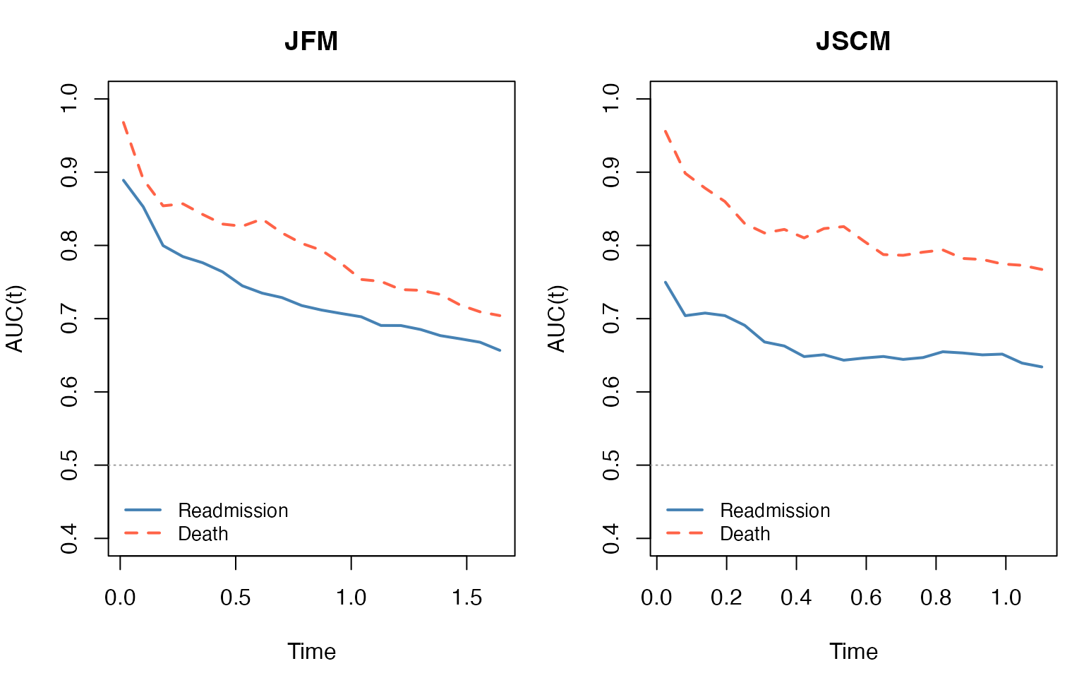


par(old_par)

11. References

Blanche, P., Dartigues, J.-F., and Jacqmin-Gadda, H. (2013). Estimating and comparing time-dependent areas under receiver operating characteristic curves for censored event times with competing risks. Statistics in Medicine, 32(30), 5381–5397.

Kalbfleisch, J. D., Schaubel, D. E., Ye, Y., and Gong, Q. (2013). An estimating function approach to the analysis of recurrent and terminal events. Biometrics, 69(2), 366–374.

Xu, G., Chiou, S. H., Huang, C.-Y., Wang, M.-C., and Yan, J. (2017). Joint scale-change models for recurrent events and failure time. Journal of the American Statistical Association, 112(518), 794–805.

Huo, L., Jiang, Z., Hou, J., and Huling, J. D. (2025). A stagewise selection framework for joint models for semi-competing risk prediction. Manuscript.

Lingfeng Huo, Ziren Jiang, Jue Hou, Jared D. Huling

2026-04-05