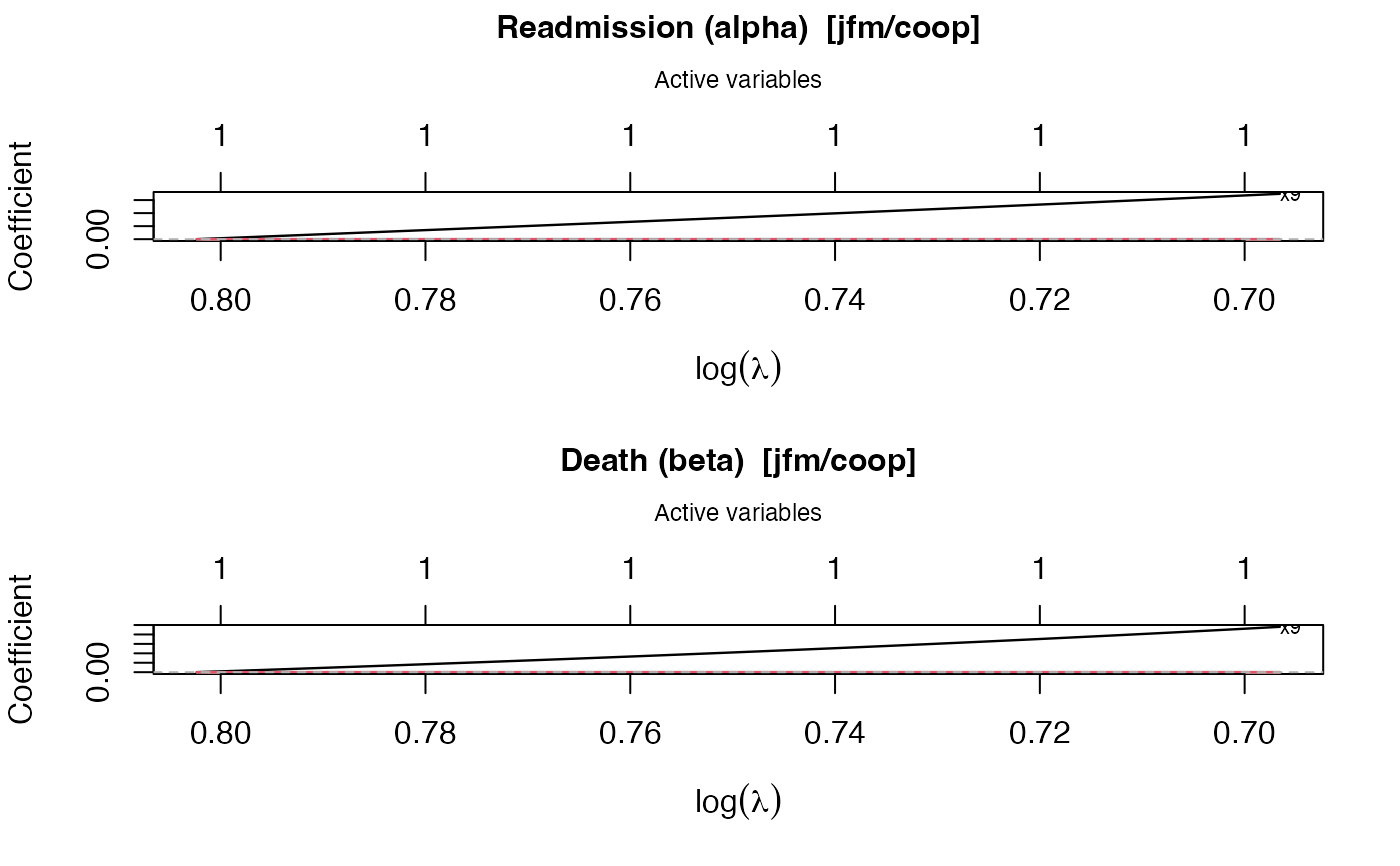
Plot a Stagewise Coefficient Path — plot.swjm

Produces a glmnet-style plot of coefficient trajectories versus \(\log(\lambda)\) along the stagewise regularization path. Two panels are drawn by default: one for the readmission sub-model (alpha) and one for the death sub-model (beta). The top axis of each panel shows the number of active variables at that lambda.

Usage

# S3 method for class 'swjm_path'
plot(
  x,
  log_lambda = TRUE,
  which = c("both", "readmission", "death"),
  col = NULL,
  ...
)

Arguments

x: An object of class "swjm_path".
log_lambda: Logical. If TRUE (default), the x-axis is \(\log(\lambda)\); otherwise raw \(\lambda\).
which: Character. Which sub-model(s) to plot: "both" (default), "readmission", or "death".
col: Optional vector of colors, one per covariate. Recycled if shorter than p.
...: Currently unused.

Value

Invisibly returns x.

Examples

# \donttest{
dat <- generate_data(n = 50, p = 10, scenario = 1, model = "jfm")
fit <- stagewise_fit(dat$data, model = "jfm", penalty = "coop",
                     max_iter = 200)
plot(fit)

# }