Plot Predicted Survival Curves and Predictor Contributions
plot.swjm_pred.RdProduces a figure for a "swjm_pred" object. The layout depends on
the model:
Arguments
- x
An object of class
"swjm_pred".- which_subject
Integer. Index of the subject to highlight (default
1).- which_process
Character. Which sub-model(s) to plot:
"both"(default),"readmission", or"death".- threshold
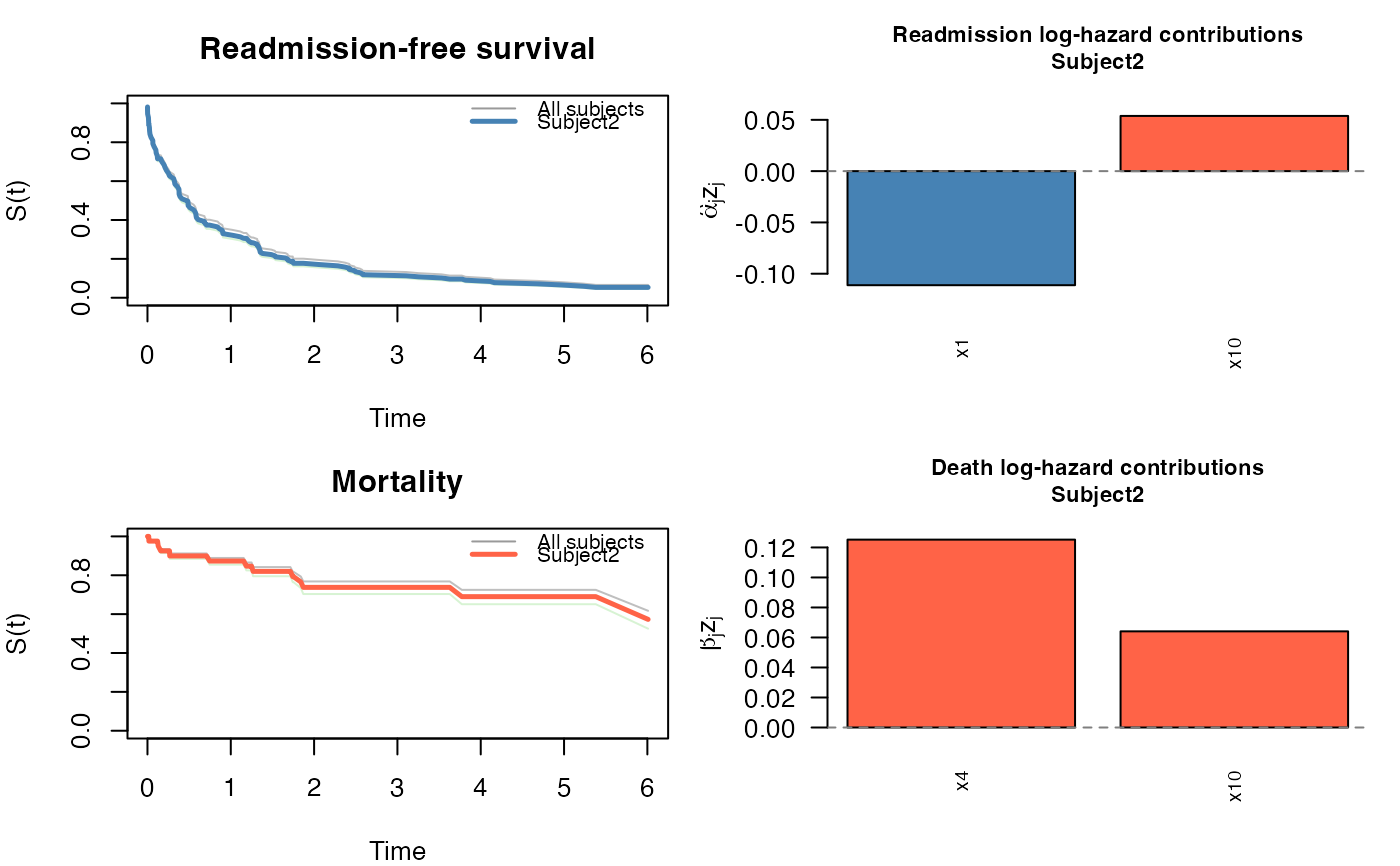
Non-negative numeric. Only predictors whose absolute subject-specific contribution exceeds this value are shown in the bar chart. The default
0suppresses variables with exactly zero contribution (i.e., unselected variables whose coefficient is zero). Increasethresholdto focus on the most impactful predictors.- ...
Currently unused.
Details
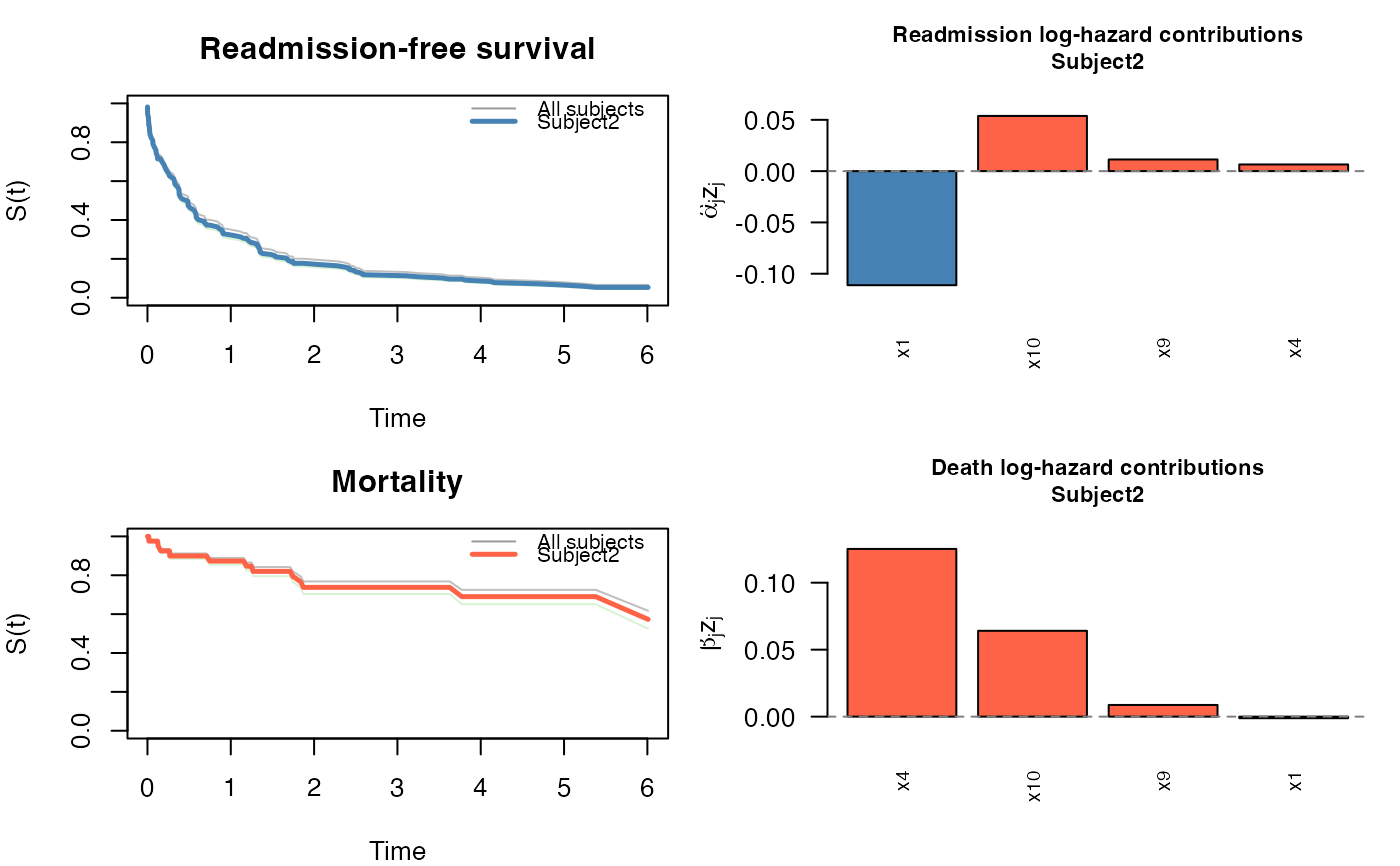
JFM (four panels):
Readmission-free survival curves for all subjects, with the selected subject highlighted.
Bar chart of readmission predictor contributions \(\hat\alpha_j z_{ij}\) (log-hazard scale).
Death-free survival curves with the selected subject highlighted.
Bar chart of death predictor contributions \(\hat\beta_j z_{ij}\).
JSCM (four panels):
Recurrent-event survival curves (AFT model) with the selected subject highlighted. The panel title shows the total acceleration factor \(e^{\hat\alpha^\top z_i}\).
Bar chart of recurrence log time-acceleration contributions \(\hat\alpha_j z_{ij}\): positive = events sooner, negative = later.
Death-free survival curves with the selected subject highlighted, total acceleration factor \(e^{\hat\beta^\top z_i}\) in the title.
Bar chart of terminal-event log time-acceleration contributions \(\hat\beta_j z_{ij}\).
In all cases bars represent subject-specific contributions (coefficient \(\times\) covariate value), not bare coefficients, so the display correctly reflects how much each predictor shifts the log-hazard (JFM) or log time-acceleration (JSCM) for this particular subject.
Examples
# \donttest{
dat  <- generate_data(n = 50, p = 10, scenario = 1, model = "jfm")
cv   <- cv_stagewise(dat$data, model = "jfm", penalty = "coop",
                     max_iter = 100)
newz <- matrix(rnorm(30), nrow = 3, ncol = 10)
pred <- predict(cv, newdata = newz)
plot(pred, which_subject = 2)

plot(pred, which_subject = 2, threshold = 0.05)

# }
# }