Predict from a Cross-Validated Joint Model Fit

Computes subject-specific predictions from a cross-validated swjm_cv fit. The output differs by model:

Usage

# S3 method for class 'swjm_cv'
predict(object, newdata, times = NULL, ...)

Arguments

object: An object of class "swjm_cv".
newdata: A numeric matrix or data frame of covariate values. Must have p columns named x1, ..., xp (if a data frame) or exactly p columns (if a matrix).
times: Numeric vector of evaluation times (JFM only). If NULL, the observed event times from the training data are used.
...: Currently unused.

Value

An object of class "swjm_pred", a list with:

S_re: Matrix of readmission-free survival probabilities (rows = subjects, columns = times).
S_de: Matrix of death-free survival probabilities.
times: Numeric vector of evaluation times.
lp_re: Linear predictors for readmission ($\hat\alpha^\top z_i$). For JSCM this is the log time-acceleration for the recurrence process.
lp_de: Linear predictors for death ($\hat\beta^\top z_i$). For JSCM this is the log time-acceleration for the terminal process.
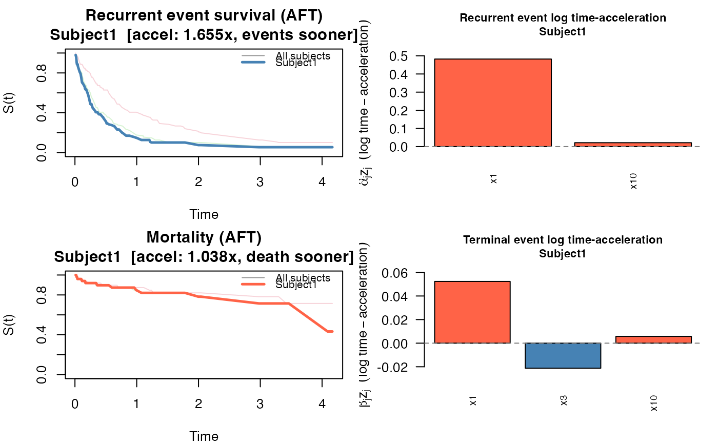
time_accel_re: (JSCM only) $e^{\hat\alpha^\top z_i}$: the multiplicative factor by which the recurrence time axis is scaled relative to baseline. NULL for JFM.
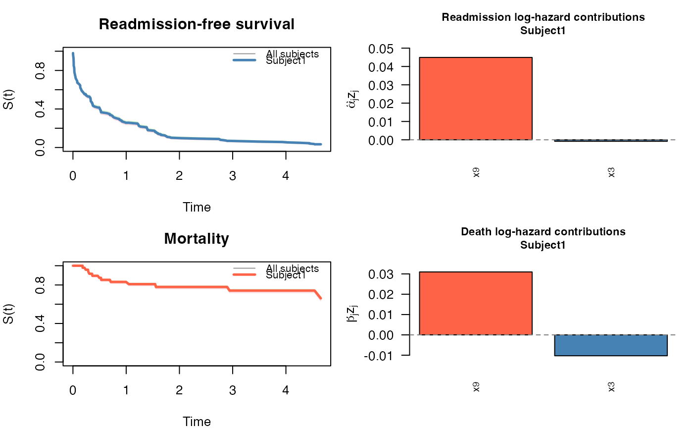
time_accel_de: (JSCM only) Analogous time-acceleration factor for the terminal process. NULL for JFM.
contrib_re: Matrix of per-predictor contributions $\hat\alpha_j z_{ij}$ (rows = subjects, columns = covariates). For JFM these are log-hazard contributions; for JSCM they are log time-acceleration contributions.
contrib_de: Analogous matrix for the terminal process.

Details

JFM — returns survival curves for both processes using the Breslow cumulative baseline hazards. For subject $i$ with covariate vector $z_i$: $$ S_{\text{re}}(t \mid z_i) = \exp\!\bigl(-\hat\Lambda_0^r(t)\, e^{\hat\alpha^\top z_i}\bigr), \quad S_{\text{de}}(t \mid z_i) = \exp\!\bigl(-\hat\Lambda_0^d(t)\, e^{\hat\beta^\top z_i}\bigr). $$

JSCM — returns survival curves for both processes using a Nelson-Aalen baseline on the accelerated time scale. For subject $i$: $$ S_{\text{re}}(t \mid z_i) = \exp\!\bigl(-\hat\Lambda_0^r(t\, e^{\hat\alpha^\top z_i})\bigr), \quad S_{\text{de}}(t \mid z_i) = \exp\!\bigl(-\hat\Lambda_0^d(t\, e^{\hat\beta^\top z_i})\bigr). $$ The linear predictor $\hat\alpha^\top z_i$ is a log time-acceleration factor: the recurrence process for subject $i$ runs on a time axis scaled by $e^{\hat\alpha^\top z_i}$ relative to the baseline. Each predictor contributes $\hat\alpha_j z_{ij}$ to this log-scale factor, so $e^{\hat\alpha_j z_{ij}}$ is the multiplicative factor on the time scale attributable to predictor $j$ alone. Values greater than 1 accelerate events (shorter times); values less than 1 decelerate them (longer times).

Examples

# \donttest{
dat <- generate_data(n = 50, p = 10, scenario = 1, model = "jfm")
cv  <- cv_stagewise(dat$data, model = "jfm", penalty = "coop",
                    max_iter = 100)
newz <- matrix(rnorm(30), nrow = 3, ncol = 10)
pred <- predict(cv, newdata = newz)
plot(pred)


dat_jscm <- generate_data(n = 50, p = 10, scenario = 1, model = "jscm")
#> Call: 
#> reReg::simGSC(n = n, summary = TRUE, para = para, xmat = X, censoring = C, 
#>     frailty = gamma, tau = 60)
#> 
#> Summary:
#> Sample size:                                    50 
#> Number of recurrent event observed:             81 
#> Average number of recurrent event per subject:  1.62 
#> Proportion of subjects with a terminal event:   0.22 
#> 
#> 
cv_jscm  <- cv_stagewise(dat_jscm$data, model = "jscm", penalty = "coop",
                          max_iter = 500)
pred_jscm <- predict(cv_jscm, newdata = newz)
plot(pred_jscm)

# }