Multi-category Treatments with personalized

Jared Huling

2022-07-07

Example with multi-category treatments

To demonstrate how to use the personalized package with multi-category treatments, we simulate data with three treatments. The treatment assignments will be based on covariates and hence mimic an observational setting with no unmeasured confounders.

library(personalized)

set.seed(123)
n.obs  <- 250
n.vars <- 10
x <- matrix(rnorm(n.obs * n.vars, sd = 3), n.obs, n.vars)

# simulated non-randomized treatment with multiple levels
# based off of a multinomial logistic model
xbetat_1 <- 0.1 + 0.5 * x[,1]  - 0.25 * x[,5]
xbetat_2 <- 0.1 - 0.5 * x[,9] + 0.25 * x[,5]
trt.1.prob <- exp(xbetat_1) / (1 + exp(xbetat_1) + exp(xbetat_2))
trt.2.prob <- exp(xbetat_2) / (1 + exp(xbetat_1) + exp(xbetat_2))
trt.3.prob <- 1 - (trt.1.prob + trt.2.prob)

prob.mat <- cbind(trt.1.prob, trt.2.prob, trt.3.prob)
trt.mat <- apply(prob.mat, 1, function(rr) rmultinom(1, 1, prob = rr))
trt.num <- apply(trt.mat, 2, function(rr) which(rr == 1))
trt <- as.factor(paste0("Trt_", trt.num))

# simulate response

# effect of treatment 1 relative to treatment 3
delta1 <- 2 * (0.5 + x[,2] - 2 * x[,3]  )
# effect of treatment 2 relative to treatment 3
delta2 <- (0.5 + x[,6] - 2 * x[,5] )

# main covariate effects with nonlinearities
xbeta <- x[,1] + x[,9] - 2 * x[,4]^2 + x[,4] + 
    0.5 * x[,5] ^ 2 + 2 * x[,2] - 3 * x[,5]

# create entire functional form of E(Y|T,X)
xbeta <- xbeta + 
    delta1 * ((trt.num == 1) - (trt.num == 3) ) + 
    delta2 * ((trt.num == 2) - (trt.num == 3) )


# simulate continuous outcomes E(Y|T,X)
y <- xbeta + rnorm(n.obs, sd = 2)

We will use the version of the treatment status vector in our analysis, however, the integer values vector, i.e. , could be used as well.

trt[1:5]

## [1] Trt_3 Trt_3 Trt_1 Trt_1 Trt_1
## Levels: Trt_1 Trt_2 Trt_3

table(trt)

## trt
## Trt_1 Trt_2 Trt_3 
##    97    86    67

Then we construct a propensity score function that takes covariate information and the treatment statuses as input and generate a matrix of probabilities as output. Each row \(i\) of the output matrix represents an observation and each column \(j\) is the probability that the \(i\)th patient received the \(j\)th treatment. The treatment levels are ordered alphabetically (or numerically if the treatment assignment vector is a vector of integers). Our propensity score model in this example will be a multinomial logistic regression model with a lasso penalty for the probability of treatment assignments conditional on covariate information:

propensity.multinom.lasso <- function(x, trt)
{
    if (!is.factor(trt)) trt <- as.factor(trt)
    gfit <- cv.glmnet(y = trt, x = x, family = "multinomial",
                      nfolds = 3)

    # predict returns a matrix of probabilities:
    # one column for each treatment level
    propens <- drop(predict(gfit, newx = x, 
        type = "response", s = "lambda.min"))

    # return the matrix probability of treatment assignments
    probs <- propens[,match(levels(trt), colnames(propens))]

    probs
}

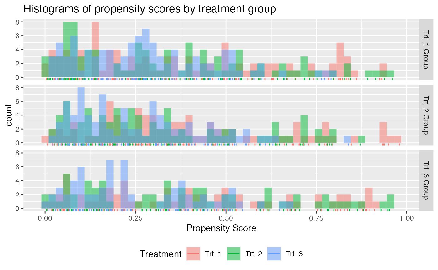
An important assumption for the propensity score is that \(0 < Pr(T_i = t | \mathbf X) < 1\) for all \(\mathbf X\) and \(t\). This assumption, often called the positivity assumption, is impossible to verify. However, in practice validity of the assumption can be assessed via a visualization of the empirical overlap of our estimated propensity scores to determine if there is any evidence of positivity violations. The function also allows us to visualize the overlap of our propensity scores for multi-category treatment applications. The following code results in the plot shown Figure \(\ref{fig:check_overlap_multitreat}\).

check.overlap(x = x, trt = trt, propensity.multinom.lasso)

Propensity score overlap plot for multi-category treatment data.

Each plot above is for a different treatment group, e.g. the plot in the first row of plots is the subset of patients who received treatment 1. There seems to be no obvious evidence against the positivity assumption.

As the outcome is continuous and there is a large number of covariates available for our construction of a benefit score, we will use the squared error loss and a lasso penalty. The model can be fit in the same manner as for the binary treatment setting, however only linear models and the weighting method are available. Here we can also specify the reference treatment (the treatment that the non-reference treatments are compared with by each benefit score).

set.seed(123)
subgrp.multi <- fit.subgroup(x = x, y = y,
    trt = trt, propensity.func = propensity.multinom.lasso,
    reference.trt = "Trt_3",
    loss   = "sq_loss_lasso",
    nfolds = 3)

summary(subgrp.multi)

## family:    gaussian 
## loss:      sq_loss_lasso 
## method:    weighting 
## cutpoint:  0 
## propensity 
## function:  propensity.func 
## 
## benefit score: f_Trt_1(x): Trt_1 vs Trt_3,  f_Trt_2(x): Trt_2 vs Trt_3 
##                f_Trt_3(x): 0 
## maxval = max(f_Trt_1(x), f_Trt_2(x)) 
## which.max(maxval) = The trt level which maximizes maxval
## Trt recom = which.max(maxval)*I(maxval > c) + Trt_3*I(maxval <= c) where c is 'cutpoint'
## 
## Average Outcomes:
##                Recommended Trt_1 Recommended Trt_2 Recommended Trt_3
## Received Trt_1  -8.2279 (n = 97)       NaN (n = 0)       NaN (n = 0)
## Received Trt_2 -22.7982 (n = 86)       NaN (n = 0)       NaN (n = 0)
## Received Trt_3 -15.5278 (n = 67)       NaN (n = 0)       NaN (n = 0)
## 
## Treatment effects conditional on subgroups:
## Est of E[Y|T=Trt_1,Recom=Trt_1]-E[Y|T=/=Trt_1,Recom=Trt_1] 
##                                          10.8514 (n = 250) 
## Est of E[Y|T=Trt_2,Recom=Trt_2]-E[Y|T=/=Trt_2,Recom=Trt_2] 
##                                                NaN (n = 0) 
## Est of E[Y|T=Trt_3,Recom=Trt_3]-E[Y|T=/=Trt_3,Recom=Trt_3] 
##                                                NaN (n = 0) 
## 
## NOTE: The above average outcomes are biased estimates of
##       the expected outcomes conditional on subgroups. 
##       Use 'validate.subgroup()' to obtain unbiased estimates.
## 
## ---------------------------------------------------
## 
## Benefit score 1 quantiles (f(X) for Trt_1 vs Trt_3): 
##   0%  25%  50%  75% 100% 
## 7.17 7.17 7.17 7.17 7.17 
## 
## Benefit score 2 quantiles (f(X) for Trt_2 vs Trt_3): 
##       0%      25%      50%      75%     100% 
## -13.2904  -8.2866  -6.5613  -5.2289   0.0758 
## 
## ---------------------------------------------------
## 
## Summary of individual treatment effects: 
## E[Y|T=trt, X] - E[Y|T=Trt_3, X]
## where 'trt' is Trt_1 and Trt_2
## 
##  Trt_1-vs-Trt_3  Trt_2-vs-Trt_3    
##  Min.   :14.34   Min.   :-26.5807  
##  1st Qu.:14.34   1st Qu.:-16.5731  
##  Median :14.34   Median :-13.1227  
##  Mean   :14.34   Mean   :-13.3502  
##  3rd Qu.:14.34   3rd Qu.:-10.4579  
##  Max.   :14.34   Max.   :  0.1516  
## 
## ---------------------------------------------------
## 
## 2 out of 20 interactions selected in total by the lasso (cross validation criterion).
## 
## The first estimate is the treatment main effect, which is always selected. 
## Any other variables selected represent treatment-covariate interactions.
## 
## 
## 0 out of 10 variables selected for delta 1 by the lasso (cross validation criterion).
## 
##                                       Trt_1
## Estimates for delta (Trt_1 vs Trt_3) 7.1698
## 
## 2 out of 10 variables selected for delta 2 by the lasso (cross validation criterion).
## 
##                                        Trt_2      V5      V9
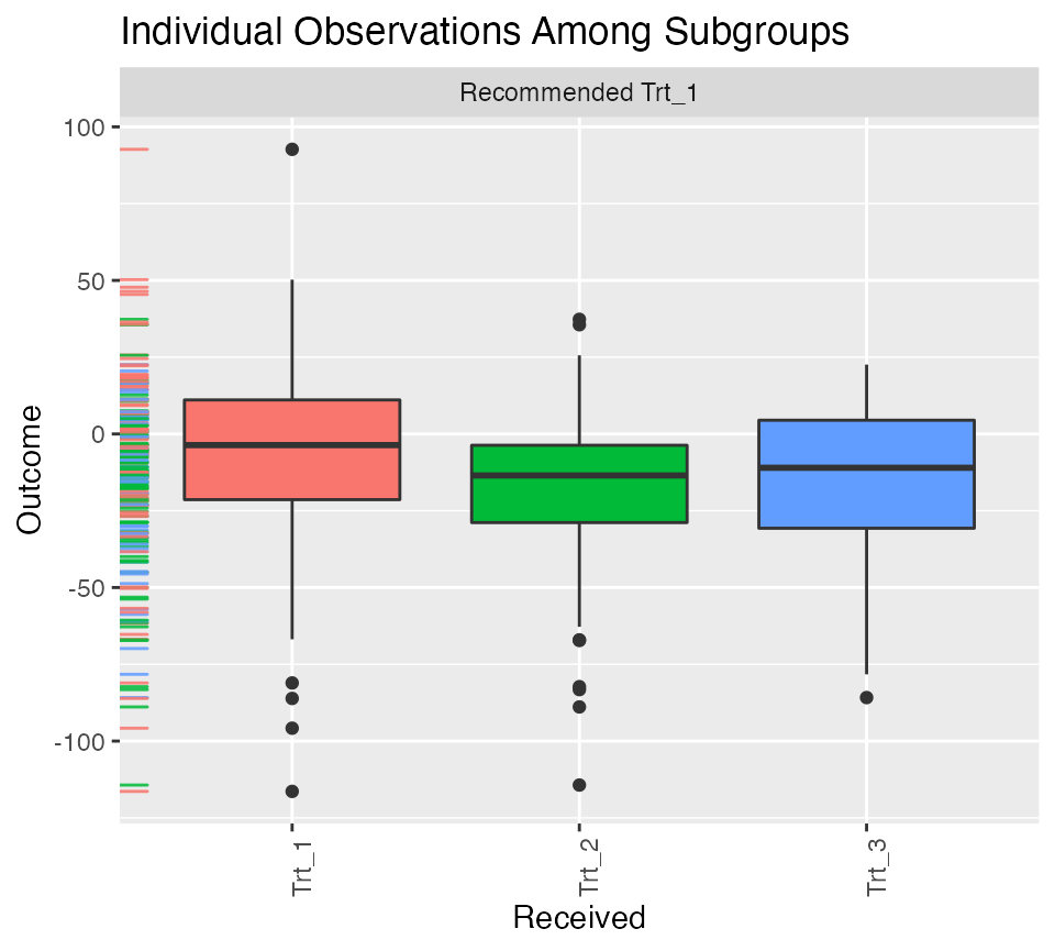
## Estimates for delta (Trt_2 vs Trt_3) -6.9472 -0.0497 -0.9131

The function now displays selected variables for each of the two benefit scores and shows the quantiles of each benefit score. We can also plot the empirical observations within the different subgroups using the function, however now it is slightly more complicated. It appears that the average outcome is higher for those who received the level of the treatment they were recommended than those who received a different treatment than they were recommended. Also note that returns a object and can thus be modified by the user. The below example yields Figure \(\ref{fig:plot_multi_trt_model}\).

pl <- plot(subgrp.multi)
pl + theme(axis.text.x = element_text(angle = 90, hjust = 1))

Individual outcome observations by treatment group and subgroup.

To obtain valid estimates of the subgroup-specific treatment effects, we perform the repeated training and testing resample procedure using the function (here we set the number of replications B=4, but this should be a much larger number in practice) :

set.seed(123)
validation.multi <- validate.subgroup(subgrp.multi, 
    B = 4,  # specify the number of replications
    method = "training_test_replication",
    train.fraction = 0.5)

print(validation.multi, digits = 2, sample.pct = TRUE)

## family:  gaussian 
## loss:    sq_loss_lasso 
## method:  weighting 
## 
## validation method:  training_test_replication 
## cutpoint:           0 
## replications:       4 
## 
## benefit score: f_Trt_1(x): Trt_1 vs Trt_3,  f_Trt_2(x): Trt_2 vs Trt_3 
##                f_Trt_3(x): 0 
## maxval = max(f_Trt_1(x), f_Trt_2(x)) 
## which.max(maxval) = The trt level which maximizes maxval
## Trt recom = which.max(maxval)*I(maxval > c) + Trt_3*I(maxval <= c) where c is 'cutpoint'
## 
## Average Test Set Outcomes:
##                       Recommended Trt_1        Recommended Trt_2
## Received Trt_1 -2.86 (SE = 1.35, 22.6%)  -2.54 (SE = 9.3, 13.4%)
## Received Trt_2 -25.56 (SE = 13.08, 24%)  -6.8 (SE = 32.93, 9.2%)
## Received Trt_3   -15.41 (SE = 2.1, 16%) -25.13 (SE = 7.82, 7.8%)
##                       Recommended Trt_3
## Received Trt_1 -36.2 (SE = 10.77, 3.2%)
## Received Trt_2 -43.89 (SE = 25.4, 2.4%)
## Received Trt_3 -21.62 (SE = 9.74, 1.4%)
## 
## Treatment effects conditional on subgroups:
## Est of E[Y|T=Trt_1,Recom=Trt_1]-E[Y|T=/=Trt_1,Recom=Trt_1] 
##                                    18.38 (SE = 6.9, 62.6%) 
## Est of E[Y|T=Trt_2,Recom=Trt_2]-E[Y|T=/=Trt_2,Recom=Trt_2] 
##                                    5.1 (SE = 29.95, 30.4%) 
## Est of E[Y|T=Trt_3,Recom=Trt_3]-E[Y|T=/=Trt_3,Recom=Trt_3] 
##                                      19.33 (SE = 9.61, 7%) 
## 
## Est of 
## E[Y|Trt received = Trt recom] - E[Y|Trt received =/= Trt recom]:                 
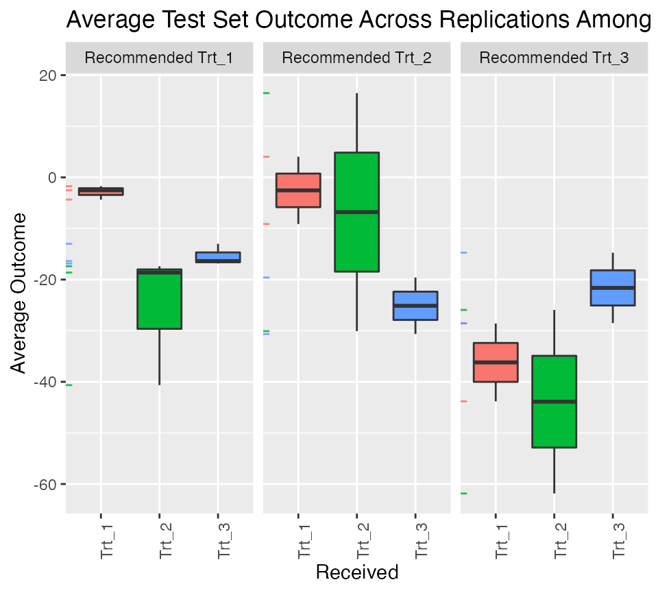
## 8.3 (SE = 16.44)

Setting the argument above to prints out the average percent of all patients which are in each subgroup (as opposed to the average sample sizes). We can see that about 58% of patients were recommended treatment 1 and among those recommended treatment 1, we expect them to have larger outcomes if they actually receive treatment 1 as opposed to the other treatments. The estimated effects are positive within all three subgroups (meaning those recommended each of the different treatments have a positive benefit from receiving the treatment they are recommended as opposed to receiving any another treatments).

We can visualize the subgroup-specific treatment effects using as usual with results shown in Figure \(\ref{fig:plotcomparemultivalidated}\):

plv <- plot(validation.multi)
plv + theme(axis.text.x = element_text(angle = 90, hjust = 1))

Validation results for multi-category treatment data.

More details on propensity scores for multi-category treatments

For cases with multi-category treatments, the user must specify a propensity function that returns \(Pr(T = T_i | \mathbf X= \mathbf x)\) for patient \(i\). In other words, it should return the probability of receiving the treatment that was actually received for each patient. For example:

propensity.func.multinom <- function(x, trt)
{
    df <- data.frame(trt = trt, x)
    mfit <- nnet::multinom(trt ~ . -trt, data = df)
    # predict returns a matrix of probabilities:
    # one column for each treatment level
    propens <- nnet::predict.nnet(mfit, type = "probs")

    if (is.factor(trt))
    {
        values <- levels(trt)[trt]
    } else 
    {
        values <- trt
    }
    # return the probability corresponding to the
    # treatment that was observed
    probs <- propens[cbind(1:nrow(propens), 
        match(values, colnames(propens)))]
    probs
}

Optionally the user can specify the function to return a matrix of treatment probabilities, however, the columns must be ordered by the levels of . An example of this is the following:

propensity.func.multinom <- function(x, trt)
{
    require(nnet)
    df <- data.frame(trt = trt, x)
    mfit <- multinom(trt ~ . -trt, data = df)
    # predict returns a matrix of probabilities:
    # one column for each treatment level
    propens <- predict(mfit, type = "probs")

    if (is.factor(trt))
    {
        levels <- levels(trt)
    } else 
    {
        levels <- sort(unique(trt))
    }
    # return the probability corresponding to the
    # treatment that was observed
    probs <- propens[,match(levels, colnames(propens))]
    probs
}