Plotting results for fitted subgroup identification models

Plots results for estimated subgroup treatment effects

Plots validation results for estimated subgroup treatment effects

# S3 method for subgroup_fitted
plot(
  x,
  type = c("boxplot", "density", "interaction", "conditional"),
  avg.line = TRUE,
  ...
)

# S3 method for subgroup_validated
plot(
  x,
  type = c("boxplot", "density", "interaction", "conditional", "stability"),
  avg.line = TRUE,
  ...
)

Arguments

x: fitted object returned by validate.subgroup() or fit.subgroup() function
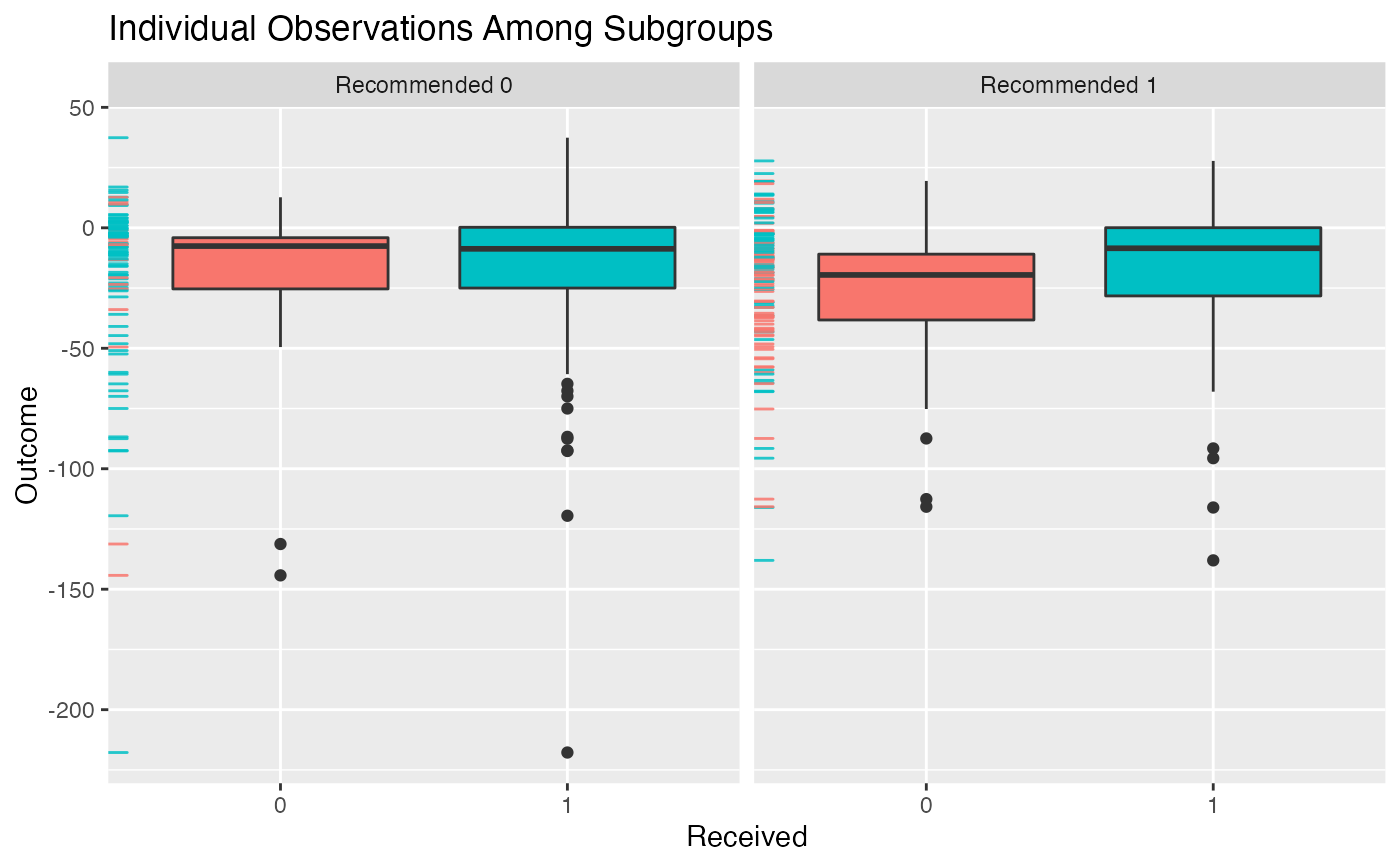
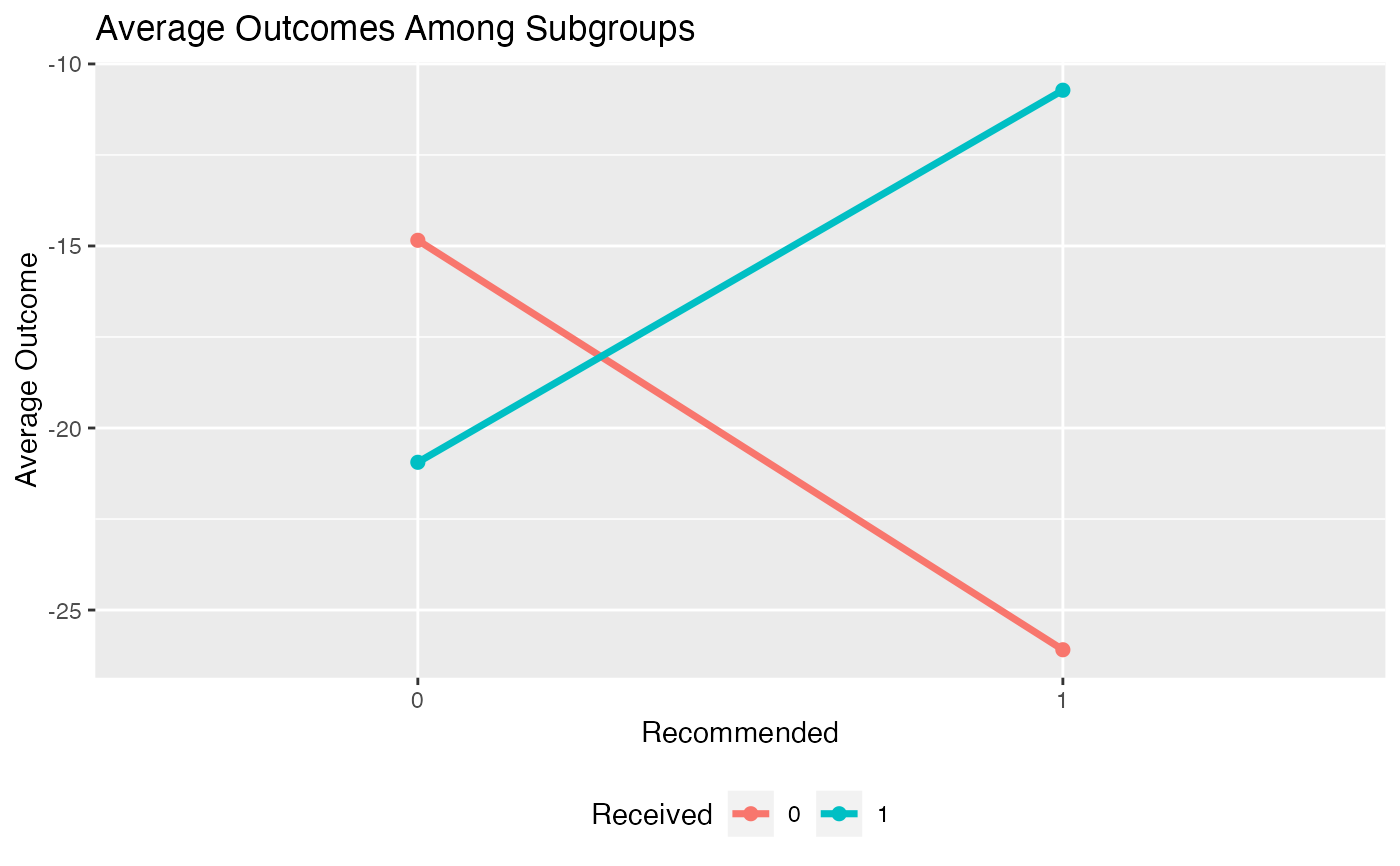
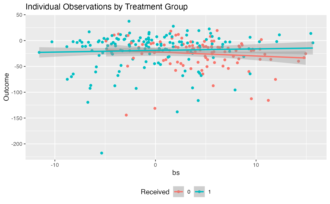
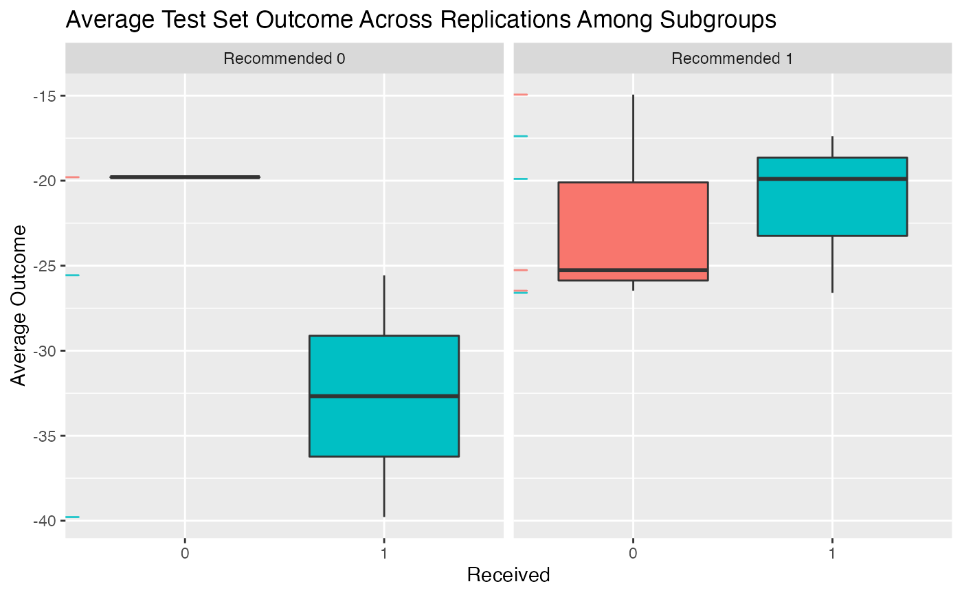
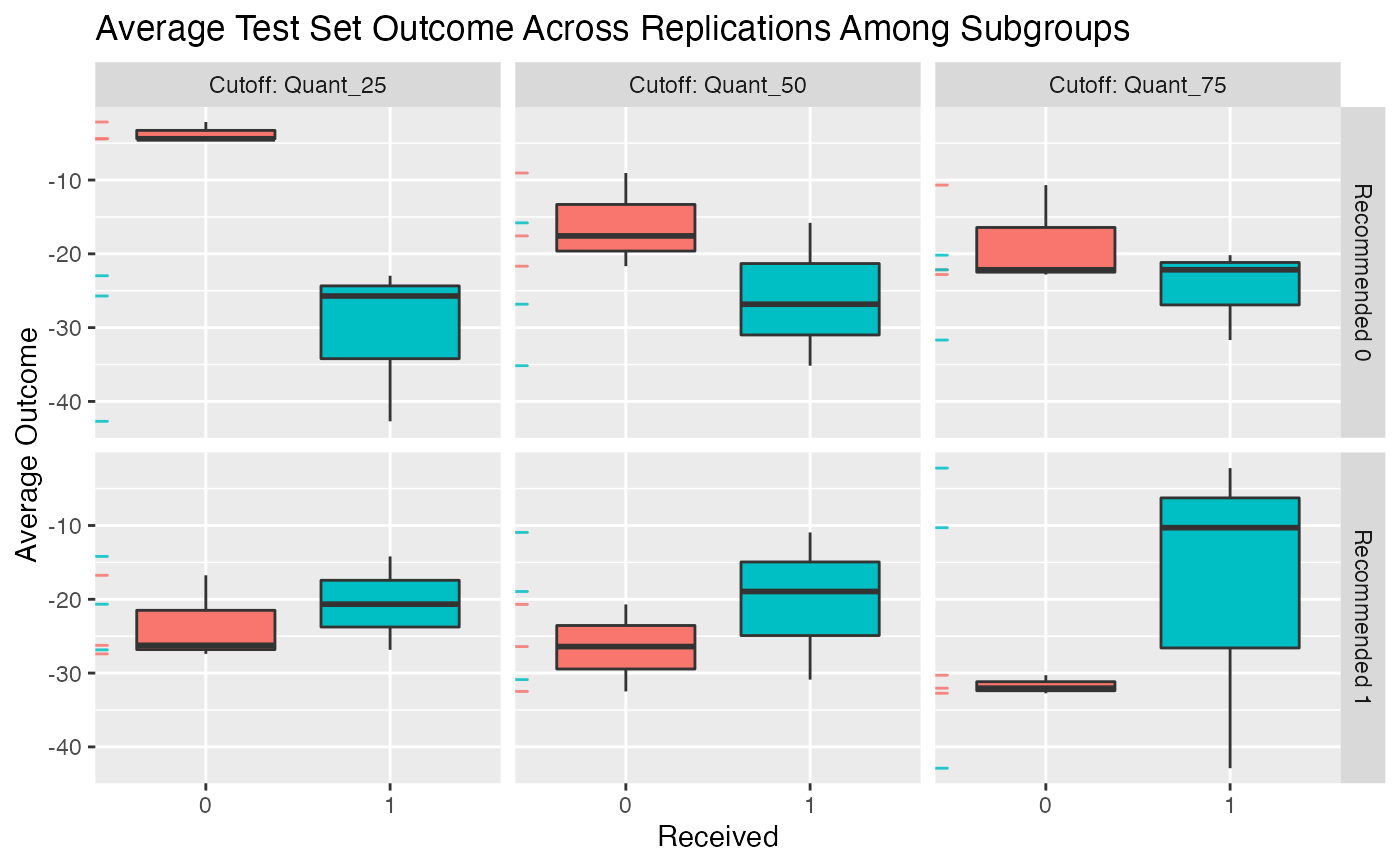
type: type of plot. "density" results in a density plot for the results across all observations (if x is from fit.subgroup()) or if x is from validate.subgroup() across iterations of either the bootstrap or training/test re-fitting. For the latter case the test results will be plotted. "boxplot" results in boxplots across all observations/iterations of either the bootstrap or training/test re-fitting. For the latter case the test results will be plotted. "interaction" creates an interaction plot for the different subgroups (crossing lines here means a meaningful subgroup). For the interaction plot, the intervals around each point represent +1 one SE "conditional" For subgroup_fitted objects, plots smoothed (via a GAM smoother) means of the outcomes as a function of the estimated benefit score separately for the treated and untreated groups. For subgroup_validated objects, boxplots of summary statistics within subgroups will be plotted as subgroups are defined by different cutoffs of the benefit scores. These cutoffs can be specified via the benefit.score.quantiles argument of validate.subgroup.
avg.line: boolean value of whether or not to plot a line for the average value in addition to the density (only valid for type = "density")
...: not used

Examples

library(personalized)

set.seed(123)
n.obs  <- 250
n.vars <- 15
x <- matrix(rnorm(n.obs * n.vars, sd = 3), n.obs, n.vars)


# simulate non-randomized treatment
xbetat   <- 0.5 + 0.5 * x[,11] - 0.5 * x[,13]
trt.prob <- exp(xbetat) / (1 + exp(xbetat))
trt01    <- rbinom(n.obs, 1, prob = trt.prob)

trt      <- 2 * trt01 - 1

# simulate response
delta <- 2 * (0.5 + x[,2] - x[,3] - x[,11] + x[,1] * x[,12])
xbeta <- x[,1] + x[,11] - 2 * x[,12]^2 + x[,13]
xbeta <- xbeta + delta * trt

# continuous outcomes
y <- drop(xbeta) + rnorm(n.obs, sd = 2)

# create function for fitting propensity score model
prop.func <- function(x, trt)
{
    # fit propensity score model
    propens.model <- cv.glmnet(y = trt,
                               x = x, family = "binomial")
    pi.x <- predict(propens.model, s = "lambda.min",
                    newx = x, type = "response")[,1]
    pi.x
}

subgrp.model <- fit.subgroup(x = x, y = y,
                           trt = trt01,
                           propensity.func = prop.func,
                           loss   = "sq_loss_lasso",
                           # option for cv.glmnet,
                           # better to use 'nfolds=10'
                           nfolds = 3)              # option for cv.glmnet

subgrp.model$subgroup.trt.effects
#> $subgroup.effects
#> Est of E[Y|T=0,Recom=0]-E[Y|T=/=0,Recom=0] 
#>                                    6.09734 
#> Est of E[Y|T=1,Recom=1]-E[Y|T=/=1,Recom=1] 
#>                                   15.36869 
#> 
#> $avg.outcomes
#>            Recommended 0 Recommended 1
#> Received 0     -14.84435     -26.09056
#> Received 1     -20.94169     -10.72186
#> 
#> $sample.sizes
#>            Recommended 0 Recommended 1
#> Received 0            17            82
#> Received 1            84            67
#> 
#> $overall.subgroup.effect
#> [1] 11.86083
#> 

plot(subgrp.model)


plot(subgrp.model, type = "boxplot")


plot(subgrp.model, type = "interaction")


plot(subgrp.model, type = "conditional")
#> `geom_smooth()` using formula 'y ~ s(x, bs = "cs")'


valmod <- validate.subgroup(subgrp.model, B = 3,
                          method = "training_test",
                          benefit.score.quantiles = c(0.25, 0.5, 0.75),
                          train.fraction = 0.75)

plot(valmod)



plot(valmod, type = "interaction")


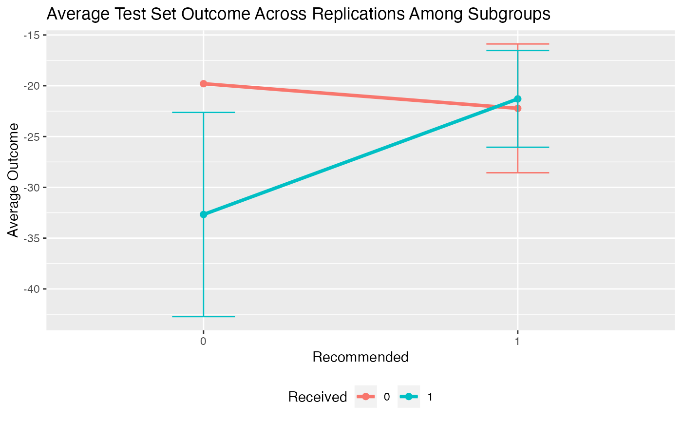# see how summary statistics of subgroups change
# when the subgroups are defined based on different cutoffs
# (25th quantile of bene score, 50th, and 75th)
plot(valmod, type = "conditional")


# visualize the frequency of particular variables
# of being selected across the resampling iterations with
# 'type = "stability"'
# not run:
# plot(valmod, type = "stability")

Arguments

See also

Examples