Plot a comparison results for fitted or validated subgroup identification models

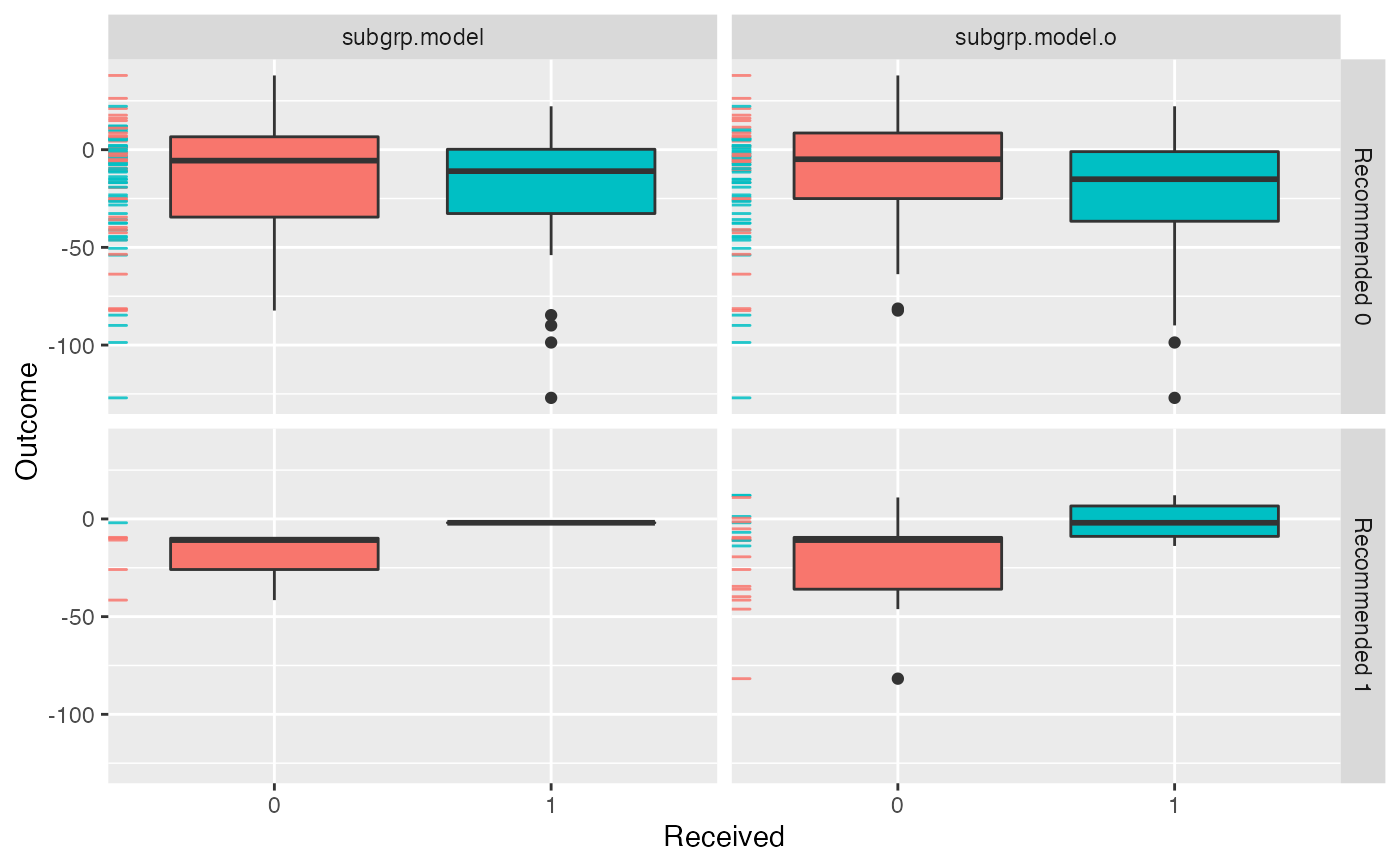
Plots comparison of results for estimated subgroup treatment effects

plotCompare(
  ...,
  type = c("boxplot", "density", "interaction", "conditional"),
  avg.line = TRUE
)

Arguments

...: the fitted (model or validation) objects to be plotted. Must be either objects returned from fit.subgroup() or validate.subgroup()
type: type of plot. "density" results in a density plot for the results across all observations (if x is from fit.subgroup()) or if x is from validate.subgroup() across iterations of either the bootstrap or training/test re-fitting. For the latter case the test results will be plotted. "boxplot" results in boxplots across all observations/iterations of either the bootstrap or training/test re-fitting. For the latter case the test results will be plotted. "interaction" creates an interaction plot for the different subgroups (crossing lines here means a meaningful subgroup). "conditional" plots smoothed (via a GAM smoother) means of the outcomes as a function of the estimated benefit score separately for the treated and untreated groups.
avg.line: boolean value of whether or not to plot a line for the average value in addition to the density (only valid for type = "density")

Examples

library(personalized)

set.seed(123)
n.obs  <- 100
n.vars <- 15
x <- matrix(rnorm(n.obs * n.vars, sd = 3), n.obs, n.vars)


# simulate non-randomized treatment
xbetat   <- 0.5 + 0.5 * x[,1] - 0.5 * x[,4]
trt.prob <- exp(xbetat) / (1 + exp(xbetat))
trt01    <- rbinom(n.obs, 1, prob = trt.prob)

trt      <- 2 * trt01 - 1

# simulate response
delta <- 2 * (0.5 + x[,2] - x[,3] - x[,11] + x[,1] * x[,12])
xbeta <- x[,1] + x[,11] - 2 * x[,12]^2 + x[,13]
xbeta <- xbeta + delta * trt

# continuous outcomes
y <- drop(xbeta) + rnorm(n.obs, sd = 2)

# create function for fitting propensity score model
prop.func <- function(x, trt)
{
    # fit propensity score model
    propens.model <- cv.glmnet(y = trt,
                               x = x, family = "binomial")
    pi.x <- predict(propens.model, s = "lambda.min",
                    newx = x, type = "response")[,1]
    pi.x
}

subgrp.model <- fit.subgroup(x = x, y = y,
                           trt = trt01,
                           propensity.func = prop.func,
                           loss   = "sq_loss_lasso",
                           # option for cv.glmnet,
                           # better to use 'nfolds=10'
                           nfolds = 3)              # option for cv.glmnet


subgrp.model.o <- fit.subgroup(x = x, y = y,
                           trt = trt01,
                           propensity.func = prop.func,
                           # option for cv.glmnet,
                           # better to use 'nfolds=10'
                           loss   = "owl_logistic_flip_loss_lasso",
                           nfolds = 3)

plotCompare(subgrp.model, subgrp.model.o)

Plot a comparison results for fitted or validated subgroup identification models

Arguments

See also

Examples