Performance and Scalability

Overview

This vignette benchmarks the forestBalance pipeline to characterize how speed and memory scale with sample size ( $n$ ) and number of trees ( $B$ ).

The pipeline has four stages, each optimized:

Forest fitting (grf::multi_regression_forest) – C++ via grf.
Leaf node extraction (get_leaf_node_matrix) – C++ via Rcpp.
Indicator matrix construction (leaf_node_kernel_Z) – C++ via Rcpp, building CSC sparse format directly without sorting.
Weight computation (kernel_balance) – adaptive solver:
- Direct: sparse Cholesky on treated/control sub-blocks. Preferred for smaller problems.
- CG: conjugate gradient using the factored $Z$ representation. No kernel matrix is formed. Preferred for large $n$ or dense kernels.

library(grf)
library(Matrix)

Mathematical background

The kernel energy balancing system

Given a kernel matrix $K \in \mathbb{R}^{n \times n}$ and a binary treatment vector $A \in \{0,1\}^n$ with $n_1$ treated and $n_0$ control units, the kernel energy balancing weights $w$ are obtained by solving the linear system $K_q \, w = z,$ where $K_q$ is the modified kernel and $z$ is a right-hand side vector determined by a linear constraint.

The modified kernel is defined element-wise as $K_q(i,j) = \frac{A_i \, A_j \, K(i,j)}{n_1^2} + \frac{(1-A_i)(1-A_j) \, K(i,j)}{n_0^2}.$

A critical structural observation is that $K_q(i,j) = 0$ whenever $A_i \neq A_j$ : the treated–control cross-blocks are identically zero. Therefore $K_q$ is block-diagonal: $K_q = \begin{pmatrix} K_{tt} / n_1^2 & 0 \\ 0 & K_{cc} / n_0^2 \end{pmatrix},$ where $K_{tt} = K[A{=}1,\; A{=}1]$ is the $n_1 \times n_1$ treated sub-block and $K_{cc} = K[A{=}0,\; A{=}0]$ is the $n_0 \times n_0$ control sub-block.

The right-hand side vector $b$ has a similarly separable structure. Writing $\mathbf{r} = K \mathbf{1}$ (the row sums of $K$ ), we have $b_i = \frac{A_i \, r_i}{n_1 \, n} + \frac{(1-A_i) \, r_i}{n_0 \, n}.$

The full system decomposes into two independent sub-problems:

Treated block: solve $K_{tt} \, w_t = n_1^2 \, z_t$ of size $n_1$ ,
Control block: solve $K_{cc} \, w_c = n_0^2 \, z_c$ of size $n_0$ ,

where $z_t$ and $z_c$ are the constraint-adjusted right-hand sides for each group (each requiring two preliminary solves to determine the Lagrange multiplier).

The kernel factorization

The proximity kernel is $K = Z Z^\top / B$ , where $Z$ is a sparse $n \times L$ indicator matrix ( $L = \sum_{b=1}^B L_b$ , total leaves across all trees). Each row of $Z$ has exactly $B$ nonzero entries (one per tree), so $Z$ has $nB$ nonzeros total. The $Z$ matrix is constructed in C++ directly in compressed sparse column (CSC) format, avoiding the overhead of R’s triplet sorting.

Direct solver (block Cholesky)

For moderate $n$ , we form the sub-block kernels explicitly: $K_{tt} = Z_t Z_t^\top / B, \qquad K_{cc} = Z_c Z_c^\top / B,$ where $Z_t = Z[A{=}1, \,\cdot\,]$ and $Z_c = Z[A{=}0, \,\cdot\,]$ . Each sub-block is computed via a sparse tcrossprod. The linear systems are then solved by sparse Cholesky factorization.

Computational Cost: $O(nB \cdot \bar{s})$ for the two sub-block cross-products (where $\bar{s}$ is the average leaf size), plus $O(n_1^{3/2} + n_0^{3/2})$ for sparse Cholesky (in the best case).

CG solver (matrix-free)

For large $n$ , forming $K_{tt}$ and $K_{cc}$ becomes expensive. The conjugate gradient (CG) solver avoids forming any kernel matrix by operating on the factored representation. To solve $K_{tt} \, x = r \quad \Longleftrightarrow \quad Z_t Z_t^\top x = B \, r,$ CG only needs matrix–vector products of the form $v \;\mapsto\; Z_t \bigl(Z_t^\top v\bigr),$ each costing $O(n_1 B)$ via two sparse matrix–vector multiplies. The same applies to the control block with $Z_c$ .

Here, the memory use is $O(nB)$ for $Z$ alone, versus $O(n^2)$ for the kernel. Each CG iteration costs $O(n_g B)$ (where $n_g$ is the group size). Convergence typically requires 100–200 iterations, independent of $n$ , so the total cost is $O(n_g B \cdot T_{\text{iter}})$ . Only four solves are needed (two per block), since the third right-hand side is a linear combination of the first two.

Computational Cost: $O\bigl((n_1 + n_0) \cdot B \cdot T_{\text{iter}}\bigr)$ where $T_{\text{iter}} \approx 100\text{--}200$ . This scales linearly in both $n$ and $B$ .

Block Jacobi preconditioned CG (default for large $n$ )

Plain CG can require many iterations at large $n$ . The Block Jacobi solver uses the first tree’s leaf partition to build a block-diagonal preconditioner. Each leaf block is a small dense system (~min.node.size $\times$ min.node.size) that is cheap to factor. Preconditioned CG then converges in far fewer iterations—typically 5–10 $\times$ fewer than plain CG—giving a large overall speedup.

Note: only 2 linear solves per treatment-group block are needed (not 3), because the third right-hand side is a linear combination of the first two.

Solver comparison

We compare all three solvers at $n = 10{,}000$ and $n = 25{,}000$ :

# Fit one forest per n, then time each solver on the SAME kernel system.
solver_bench <- do.call(rbind, lapply(c(10000, 25000), function(nn) {
  set.seed(123)
  dat <- simulate_data(n = nn, p = 10)
  B_val <- 1000
  mns <- max(20L, min(floor(nn / 200) + 10, floor(nn / 50)))

  forest <- grf::multi_regression_forest(
    dat$X, scale(cbind(dat$A, dat$Y)),
    num.trees = B_val, min.node.size = mns
  )
  leaf_mat <- get_leaf_node_matrix(forest, dat$X)
  Z <- leaf_node_kernel_Z(leaf_mat)

  solvers <- if (nn <= 10000) c("bj", "cg", "direct") else c("bj", "cg")
  do.call(rbind, lapply(solvers, function(s) {
    if (s == "direct") {
      K <- leaf_node_kernel(leaf_mat)
      t <- system.time(
        w <- kernel_balance(dat$A, kern = K, solver = "direct")
      )["elapsed"]
    } else {
      t <- system.time(
        w <- kernel_balance(dat$A, Z = Z, leaf_matrix = leaf_mat,
                             num.trees = B_val, solver = s)
      )["elapsed"]
    }
    ate <- weighted.mean(dat$Y[dat$A == 1], w$weights[dat$A == 1]) -
           weighted.mean(dat$Y[dat$A == 0], w$weights[dat$A == 0])
    data.frame(n = nn, solver = s, time = t, ate = ate)
  }))
}))

Solver comparison on the same kernel (B = 1,000). ATE agreement confirms solvers find the same solution.
n	Solver	Time (s)	ATE
10000	bj	5.54	0.015260
10000	cg	4.26	0.015261
10000	direct	17.39	0.015260
25000	bj	30.47	0.006337
25000	cg	40.63	0.006344

All solvers produce the same ATE to high precision, confirming they solve the same system. CG (Rcpp) is the robust default; Block Jacobi can be faster in specific regimes (moderate leaf size, many trees) and is available via solver = "bj".

End-to-end timing

We benchmark the full forest_balance() pipeline (forest fitting, leaf extraction, Z construction, and weight computation) across a range of sample sizes up to $n = 50{,}000$ with $B = 1{,}000$ trees:

n_vals <- c(500, 1000, 2500, 5000, 10000, 25000, 50000)
B <- 1000
p <- 10

bench <- do.call(rbind, lapply(n_vals, function(nn) {
  set.seed(123)
  dat <- simulate_data(n = nn, p = p)

  # Auto (default)
  t_auto <- system.time(
    fit_auto <- forest_balance(dat$X, dat$A, dat$Y, num.trees = B)
  )["elapsed"]

  data.frame(n = nn, trees = B, auto = t_auto,
             auto_solver = fit_auto$solver)
}))

Full pipeline time (auto solver).
n	Trees	Time (s)	Solver
500	1000	0.15	cg
1000	1000	0.18	direct
2500	1000	0.62	direct
5000	1000	2.20	direct
10000	1000	9.51	direct
25000	1000	38.16	cg
50000	1000	115.98	cg

plot of chunk timing-plot

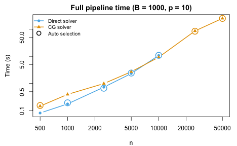
The solver is selected automatically based on the per-fold sample size. The Block Jacobi preconditioned CG (green) activates for large $n$ and provides the best scaling.

Scaling with number of trees

tree_vals <- c(200, 500, 1000, 2000)
n_test <- c(1000, 5000, 25000)

tree_bench <- do.call(rbind, lapply(n_test, function(nn) {
  do.call(rbind, lapply(tree_vals, function(B) {
    set.seed(123)
    dat <- simulate_data(n = nn, p = 10)
    t <- system.time(
      fit <- forest_balance(dat$X, dat$A, dat$Y, num.trees = B)
    )["elapsed"]
    data.frame(n = nn, trees = B, time = t)
  }))
}))

Pipeline time across tree counts.
n	Trees	Time (s)
1000	200	0.05
1000	500	0.10
1000	1000	0.17
1000	2000	0.34
5000	200	0.93
5000	500	1.30
5000	1000	2.09
5000	2000	3.97
25000	200	10.00
25000	500	23.66
25000	1000	37.66
25000	2000	66.03

plot of chunk tree-plot

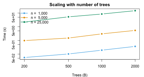
The pipeline scales approximately linearly in both $n$ and $B$ .

Pipeline stage breakdown

The following experiment profiles each stage of the pipeline individually to show where time is spent at different scales:

breakdown <- do.call(rbind, lapply(
  list(c(1000, 500), c(5000, 500), c(5000, 2000),
       c(25000, 500), c(25000, 1000)),
  function(cfg) {
    nn <- cfg[1]; B_val <- cfg[2]
    set.seed(123)
    dat <- simulate_data(n = nn, p = 10)
    mns <- max(20L, min(floor(nn / 200) + 10, floor(nn / 50)))

    # 1. Forest fitting
    t_fit <- system.time({
      resp <- scale(cbind(dat$A, dat$Y))
      forest <- grf::multi_regression_forest(dat$X, Y = resp,
                        num.trees = B_val, min.node.size = mns)
    })["elapsed"]

    # 2. Leaf extraction (Rcpp)
    t_leaf <- system.time(
      leaf_mat <- get_leaf_node_matrix(forest, dat$X)
    )["elapsed"]

    # 3. Z construction (Rcpp)
    t_z <- system.time(
      Z <- leaf_node_kernel_Z(leaf_mat)
    )["elapsed"]

    # 4. Weight computation (kernel_balance)
    t_bal <- system.time(
      w <- kernel_balance(dat$A, Z = Z, num.trees = B_val, solver = "cg")
    )["elapsed"]

    data.frame(n = nn, trees = B_val, mns = mns,
               fit = t_fit, leaf = t_leaf, Z = t_z, balance = t_bal,
               total = t_fit + t_leaf + t_z + t_bal)
  }
))

Wall-clock time for each pipeline stage across configurations (CG solver, single fold).
n	Trees	mns	Forest fit (s)	Leaf extract (s)	Z build (s)	Balance (s)	Total (s)
1000	500	20	0.03	0.02	0.004	0.10	0.15
5000	500	35	0.17	0.11	0.012	0.65	0.94
5000	2000	35	0.66	0.42	0.102	2.33	3.52
25000	500	135	0.94	0.53	0.069	26.14	27.68
25000	1000	135	1.87	1.06	0.181	41.14	44.26

plot of chunk breakdown-plot

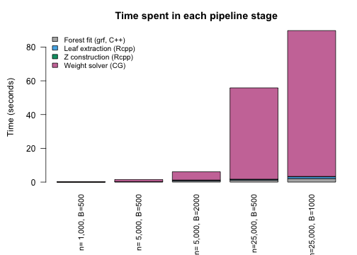
At small $n$ , forest fitting and the balance solver take similar time. At large $n$ , the CG solver dominates — its cost grows with the number of iterations and the sparse matrix–vector product size. The C++ stages (leaf extraction and $Z$ construction) remain a small fraction throughout.

Memory usage

When the direct solver is used, the kernel is formed as a sparse matrix. For the CG solver, only the sparse indicator matrix $Z$ is stored. The table below shows the actual memory usage compared to the theoretical dense kernel:

mem_data <- do.call(rbind, lapply(
  c(500, 1000, 2500, 5000, 10000, 25000, 50000),
  function(nn) {
    set.seed(123)
    dat <- simulate_data(n = nn, p = 10)
    B_val <- 1000
    mns <- max(20L, min(floor(nn / 200) + ncol(dat$X), floor(nn / 50)))

    fit_forest <- multi_regression_forest(
      dat$X, scale(cbind(dat$A, dat$Y)),
      num.trees = B_val, min.node.size = mns
    )
    leaf_mat <- get_leaf_node_matrix(fit_forest, dat$X)

    Z <- leaf_node_kernel_Z(leaf_mat)
    z_mb <- as.numeric(object.size(Z)) / 1e6

    # Kernel sparsity (skip forming K for very large n)
    if (nn <= 10000) {
      K <- leaf_node_kernel(leaf_mat)
      pct_nz <- round(100 * length(K@x) / as.numeric(nn)^2, 1)
      k_mb <- round(as.numeric(object.size(K)) / 1e6, 1)
    } else {
      pct_nz <- NA
      k_mb <- NA
    }

    n_fold <- nn %/% 2
    auto_solver <- if (n_fold > 5000 || mns > n_fold / 20) "cg" else "direct"
    dense_mb <- round(8 * as.numeric(nn)^2 / 1e6, 0)

    data.frame(n = nn, mns = mns, pct_nz = pct_nz,
               sparse_MB = k_mb, Z_MB = round(z_mb, 1),
               dense_MB = dense_mb, solver = auto_solver)
  }
))

Memory usage with adaptive leaf size (p = 10).
n	mns	Solver	K % nonzero	Stored	Actual (MB)	Dense K (MB)	Actual / Dense
500	20	cg	39.4%	Z (factor)	6.0	2	300%
1000	20	direct	28.8%	K (sparse)	3.5	8	43.8%
2500	22	direct	20.1%	K (sparse)	15.1	50	30.2%
5000	35	direct	16%	K (sparse)	48.1	200	24%
10000	60	direct	12.6%	K (sparse)	151.7	800	19%
25000	135	cg	–	Z (factor)	300.4	5000	6%
50000	260	cg	–	Z (factor)	600.3	20000	3%

plot of chunk memory-plot

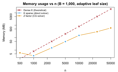
At $n = 50{,}000$ , a dense kernel would require 19 GB. The CG solver stores only the $Z$ matrix, using a small fraction of this.

Summary

The full forest_balance() pipeline scales to $n = 50{,}000$ with 1,000 trees.
All computationally intensive steps are in compiled code: C++ for leaf extraction and $Z$ construction (Rcpp), BLAS for sparse matrix operations, and CHOLMOD for sparse Cholesky.
The adaptive min.node.size heuristic adjusts leaf size to both $n$ and $p$ , creating denser kernels than the old default of 10.
The solver switchover between direct and CG depends on both the per-fold sample size and the kernel density. The "auto" setting handles this transparently.
The pipeline scales approximately linearly in both $n$ and $B$ .